Filtering of Stochastic Signals
We now have the tools necessary to describe what happens when a stochastic signal is processed through a linear, time-invariant (LTI) system. These tools consist of measures on the random signals which describe and/or characterize the signals. The two most important of these are the mean value of the signal and the autocorrelation function of the signal. Further, we can characterize the relation between two random signals through the cross-correlation function. In all of our discussions we will assume that our random processes are complex as well as ergodic (and thus stationary).
We recall that:
| (6.1) |
$$\begin{array}{*{20}{l}}
{{\varphi _{xx}}[k]}&{ = E\left\{ {x[n]\,{x^*}[n + k]} \right\}}\\
{\,\,\,}&{ = \! < x[n]\,{x^*}[n + k] > \;}\\
{\,\,\,}&\begin{array}{l}
= \mathop {\lim }\limits_{N \to \infty } \frac{1}{{2N + 1}}\sum\limits_{n = - N}^{ + N} {x[n]\,{x^*}[n + k]} \\
\,\,\,
\end{array}
\end{array}$$
|
| (6.2) |
$$\begin{array}{l}
\begin{array}{*{20}{l}}
{{\varphi _{xy}}[k]}&{ = E\left\{ {x[n]\,{y^*}[n + k]} \right\}}\\
{\,\,\,}&{ = \! < x[n]\,{y^*}[n + k] > \;}\\
{\,\,\,}&{ = \mathop {\lim }\limits_{N \to \infty } \frac{1}{{2N + 1}}\sum\limits_{n = - N}^{ + N} {x[n]\,{y^*}[n + k]} }
\end{array}\\
\,\,\,
\end{array}$$
|
| (6.3) |
$$\begin{array}{*{20}{l}}
{{m_x}}&{ = E\left\{ {x[n]} \right\} = \! < x[n] > }\\
{\,\,\,}&{ = \mathop {\lim }\limits_{N \to \infty } \frac{1}{{2N + 1}}\sum\limits_{n = - N}^{ + N} {x[n]} }
\end{array}$$
|
To understand what happens when stochastic signals are processed by LTI systems, let us begin with discrete-time convolution.
Interpretation of the convolution result
First we can say that the relation between input and output is still given by the convolution sum, that is, we can write the input as:
| (6.4) |
$$x[n] = \sum\limits_{k = - \infty }^{ + \infty } {x[k]\,\delta [n - k]}$$
|
The total signal is a weighted sum of unit impulse functions where the weights \(\left\{ {x[k]} \right\}\) have random values according to some probability function. The basic concepts of convolution theory, as argued below, still hold. As a reminder of what Equation 6.4 means, see Figure 3.1.
The deterministic impulse function \(\delta [n]\) produces the impulse response \(h[n]\) from the LTI system. A delayed version \(\delta [n - k]\) produces a delayed output \(h[n - k].\) Multiplication of the input by a scale factor produces multiplication of the output by the same factor even if that factor is a random variable.
Thus \(x[k]\,\delta [n - k]\) will produce \(x[k]\,h[n - k]\) as an output. Because the input \(x[n]\) can be expressed as the sum of inputs of this form, we can apply the linearity conditions, Equation 4.13 and Equation 4.14, to write the output as:
| (6.5) |
$$y[n] = \sum\limits_{k = - \infty }^{ + \infty } {x[k]\,h[n - k]} = x[n] \otimes h[n]$$
|
The model for this situation is shown in Figure 6.1.

It is easy to see from Equation 6.5 that \(y[n]\) will be a stochastic signal if \(x[n]\) is a stochastic signal. The questions now arise:
- If the input mean is \({m_x},\) what is the output mean \({m_y}?\)
- If the input autocorrelation function is \({\varphi _{xx}}[k],\) what form does the output autocorrelation function \({\varphi _{yy}}[k]\) have?
- Assuming that the input is stationary, is the output also stationary?
The mean
Using the standard definition we have:
| (6.6) |
$$\begin{array}{*{20}{l}}
{{m_y}}&{ = E\left\{ {y[n]} \right\} = E\left\{ {\sum\limits_{k = - \infty }^{ + \infty } {x[k]\,h[n - k]} } \right\}}\\
{\,\,\,}&{ = \sum\limits_{k = - \infty }^{ + \infty } {E\left\{ {x[k]\,h[n - k]} \right\}} }
\end{array}$$
|
This last statement is true because, as we have observed earlier in Equation 4.13, the averaging operator (or expectation operator) distributes over addition.
Only the weights \(\left\{ {x[k]} \right\}\) are random variables. The impulse response, \(h[n],\) of the LTI system is not random and the term \(h[n - k]\) is a constant with respect to the averaging process over the random variable \(x[k].\) We can, therefore, rewrite this equation as:
| (6.7) |
$${m_y} = \sum\limits_{k = - \infty }^{ + \infty } {E\left\{ {x[k]\,h[n - k]} \right\}} = \sum\limits_{k = - \infty }^{ + \infty } {E\left\{ {x[k]} \right\}\,} h[n - k]$$
|
Because the random process \(\left\{ {x[k]} \right\}\) is stationary (independent of \(n\)) we have:
| (6.8) |
$$\begin{array}{*{20}{l}}
{{m_y}}&{ = \sum\limits_{k = - \infty }^{ + \infty } {E\left\{ {x[k]} \right\}h[n - k]} = \sum\limits_{k = - \infty }^{ + \infty } {{m_x}h[n - k]} }\\
{\,\,\,}&{ = {m_x}\sum\limits_{k = - \infty }^{ + \infty } {h[n - k]} }
\end{array}$$
|
Using the Fourier transform of the impulse response \(H(\Omega ) = {\mathscr{F}}\left\{ {h[n]} \right\}\) (Equation 3.3), this expression simplifies to:
| (6.9) |
$$\begin{array}{*{20}{l}}
{{m_y}}&{ = {m_x}\sum\limits_{k = - \infty }^{ + \infty } {h[n - k]} = {m_x}\sum\limits_{n = - \infty }^{ + \infty } {h[n]} }\\
{\,\,\,}&{ = {m_x}H(\Omega = 0)}
\end{array}$$
|
What does this mean? From our knowledge of LTI filter theory, the expression \({m_y} = {m_x}H(\Omega = 0)\) makes sense. The expression says the average value of the input random signal is multiplied by the constant gain factor—the gain at (\(\Omega = 0\))—of the linear filter. Because the average value is, indeed, just a constant (DC) value, the non-fluctuating component, this is a realistic result. Note that \(H(\Omega ),\) \({m_x}\) and \({m_y}\) are all complex in this derivation.
We also see through this derivation that, because the input average is stationary, the output average is also stationary.
The autocorrelation function
The development of the output correlation proceeds along similar lines:
| (6.10) |
$$\begin{array}{l}
{\varphi _{yy}}[n,n + k] = E\left\{ {y[n]{y^*}[n + k]} \right\}\\
\,\,\,\,\,\,\,\, = E\left\{ {\left( {\sum\limits_{m = - \infty }^{ + \infty } {h[m ]x[n - m ]} } \right)\left( {\sum\limits_{r = - \infty }^{ + \infty } {{h^*}[r]{x^*}[n + k - r]} } \right)} \right\}\\
\,\,\,\,\,\,\,\, = E\left\{ {\sum\limits_{m = - \infty }^{ + \infty } {\sum\limits_{r = - \infty }^{ + \infty } {h[m ]{h^*}[r]x[n - m ]{x^*}[n + k - r]} } } \right\}
\end{array}$$
|
Using the distributive property once again:
| (6.11) |
$${\varphi _{yy}}[n,n + k] = \sum\limits_{m = - \infty }^{ + \infty } {\sum\limits_{r = - \infty }^{ + \infty } {h[m ]{h^*}[r]E\left\{ {x[n - m ]{x^*}[n + k - r]} \right\}} }$$
|
The term within the expectation braces \(E\left\{ \bullet \right\}\) yields \({\varphi _{xx}}[k + m - r]\) producing:
| (6.12) |
$${\varphi _{yy}}[n,n + k] = \sum\limits_{m = - \infty }^{ + \infty } {\sum\limits_{r = - \infty }^{ + \infty } {h[m ]{h^*}[r]{\varphi _{xx}}[k + m - r]} }$$
|
Because \(m\) and \(r\) in Equation 6.12 are simply dummy variables that disappear when the two sums are performed, the result of the double sum, \({\varphi _{yy}},\) will only be a function of \(k\) and, of course, the precise forms of the impulse response \(h[n]\) and the autocorrelation function \({\varphi _{xx}}.\)
If the right side of Equation 6.12 is only a function of \(k\) then the left side is only a function of \(k,\) as well, and we have:
| (6.13) |
$${\varphi _{yy}}[n,n + k] = {\varphi _{yy}}[k] = \sum\limits_{m = - \infty }^{ + \infty } {\sum\limits_{r = - \infty }^{ + \infty } {h[m ]{h^*}[r]{\varphi _{xx}}[k + m - r]} }$$
|
From this we can conclude that if \({\varphi _{xx}}[ \bullet ]\) is stationary then \({\varphi _{yy}}[ \bullet ]\) is stationary. We can go further. If we set \(n = r - m,\) then:
| (6.14) |
$$\begin{array}{*{20}{l}}
{{\varphi _{yy}}[k]}&{ = \sum\limits_{m = - \infty }^{ + \infty } {\sum\limits_{n = - \infty }^{ + \infty } {h[m]{h^*}[m + n]{\varphi _{xx}}[k - n]} } }\\
{\,\,\,}&{ = \sum\limits_{n = - \infty }^{ + \infty } {{\varphi _{xx}}[k - n]} \left( {\sum\limits_{m = - \infty }^{ + \infty } {h[m]{h^*}[m + n]} } \right)}
\end{array}$$
|
We recognize from ordinary (deterministic) signal processing theory that the term within parentheses is the autocorrelation of the impulse response. If this autocorrelation is \({\varphi _{hh}}[m]\) then:
| (6.15) |
$${\varphi _{yy}}[k] = \sum\limits_{m = - \infty }^{ + \infty } {{\varphi _{xx}}[k - m]} {\varphi _{hh}}[m] = {\varphi _{xx}}[k] \otimes {\varphi _{hh}}[k]$$
|
Our conclusion is that the autocorrelation of the output is stationary and is the convolution of the autocorrelation function of the (random) input signal with the autocorrelation function of the (deterministic) impulse response.
The cross-correlation function
Finally we can derive the cross-correlation between the input and output as:
| (6.16) |
$$\begin{array}{*{20}{l}}
{{\varphi _{xy}}[k]}&{ = E\left\{ {x[n]{y^*}[n + k]} \right\}}\\
{\,\,\,}&{ = E\left\{ {x[n]\left( {\sum\limits_{m = - \infty }^{ + \infty } {{h^*}[m ]{x^*}[n + k - m]} } \right)} \right\}}\\
{\,\,\,}&{ = \sum\limits_{m = - \infty }^{ + \infty } {{h^*}[m ]E\left\{ {x[n]{x^*}[n + k - m]} \right\}} }
\end{array}$$
|
Once again, the term within the expectation braces gives the stationary autocorrelation function \({\varphi _{xx}}[k - m].\) Continuing,
| (6.17) |
$${\varphi _{xy}}[k] = \sum\limits_{m = - \infty }^{ + \infty } {{h^*}[m]} {\varphi _{hh}}[k - m] = {h^*}[k] \otimes {\varphi _{xx}}[k]$$
|
The cross-correlation function is stationary and is the convolution of the complex conjugate of the (deterministic) impulse response with the autocorrelation function of the (random) input signal.
We can now express the Fourier transforms of \({\varphi _{xx}}[k]\) and \({\varphi _{yy}}[k]\) in terms of known quantities.
| (6.18) |
$$\begin{array}{*{20}{l}}
{{S_{yy}}(\Omega )}&{ = {\mathscr{F}}\left\{ {{\varphi _{yy}}[k]} \right\} = {\mathscr{F}}\left\{ {{\varphi _{xx}}[k] \otimes {\varphi _{hh}}[k]} \right\}}\\
{\,\,\,}&{ = {S_{xx}}(\Omega )\;{S_{hh}}(\Omega )}
\end{array}$$
|
But using the result from Fourier theory that \({\mathscr{F}}\left\{ {{h^*}[n]} \right\} = {H^*}\left( { - \Omega } \right)\) gives:
| (6.19) |
$$\begin{array}{*{20}{l}}
{{S_{hh}}(\Omega )}&{ = {\mathscr{F}}\left\{ {\sum\limits_{m = - \infty }^{ + \infty } {h[m]{h^*}[m + n]} } \right\}}\\
{\,\,\,}&{ = H( - \Omega )\;{H^*}( - \Omega ) = {{\left| {H( - \Omega )} \right|}^2}}
\end{array}$$
|
Therefore,
| (6.20) |
$${S_{yy}}(\Omega ) = {\left| {H( - \Omega )} \right|^2}{S_{xx}}(\Omega )$$
|
If the impulse response \(h[n]\) of the deterministic system is real, then this is equivalent to:
| (6.21) |
$${S_{yy}}(\Omega ) = {\left| {H(\Omega )} \right|^2}{S_{xx}}(\Omega )$$
|
Returning to the complex form of \(h[n],\) the cross power density spectrum can be similarly shown to be:
| (6.22) |
$${S_{xy}}(\Omega ) = {H^*}( - \Omega ){S_{xx}}(\Omega )$$
|
Again, if the impulse response \(h[n]\) of the deterministic system is real, then this is equivalent to:
| (6.23) |
$${S_{xy}}(\Omega ) = H(\Omega ){S_{xx}}(\Omega )$$
|
Based upon the use of these results we are now in a position to provide an interpretation of the power spectrum \({S_{xx}}(\Omega ).\)
We see from Equation 5.3 that for \(k = 0\):
| (6.24) |
$${\varphi _{xx}}[0] = E\left\{ {x[n]{x^*}[n]} \right\}\; = E\left\{ {{{\left| {x[n]} \right|}^2}} \right\}\; \ge 0$$
|
Similarly \({\varphi _{yy}}[k] \ge 0\) and
| (6.25) |
$$\begin{array}{*{20}{l}}
{{\varphi _{yy}}[0]}&{ = \frac{1}{{2\pi }}\int\limits_{ - \pi }^{ + \pi } {{S_{yy}}(\Omega )} d\Omega }\\
{\,\,\,}&{ = \frac{1}{{2\pi }}\int\limits_{ - \pi }^{ + \pi } {{{\left| {H( - \Omega )} \right|}^2}{S_{xx}}(\Omega )} d\Omega }
\end{array}$$
|
Let \(H(\Omega )\) be a (complex) bandpass filter (as shown in Figure 6.2) such that within the pass-band the spectrum \({S_{xx}}(\Omega )\) is essentially constant.
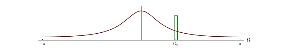
For complex random processes \({\varphi _{xx}}[k] = \varphi _{xx}^*[ - k],\) Equation 5.5, which means that \({S_{xx}}(\Omega )\) is real Equation 5.26. For a sufficiently small passband \(\Delta \Omega,\) we can write:
| (6.26) |
$$\begin{array}{*{20}{l}}
{{\varphi _{yy}}[0]}&{ = \frac{1}{{2\pi }}{S_{yy}}(\Omega = {\Omega _0})\Delta \Omega }&{ \ge 0}\\
{\,\,\,}&{ = \frac{1}{{2\pi }}{{\left| {H( - {\Omega _0})} \right|}^2}{S_{xx}}({\Omega _0})\Delta \Omega }&{ \ge 0}
\end{array}$$
|
Because \({S_{xx}}(\Omega )\) is real, we immediately have that
| (6.27) |
$${S_{xx}}({\Omega _0}) \ge 0$$
|
for all choices of \({\Omega _0}.\)
Further \({\left| {y[n]} \right|^2}\) is (by definition) the instantaneous power in a signal (including random signals) and thus \({\varphi _{yy}}[0] = E\left\{ {{{\left| {y[n]} \right|}^2}} \right\}\) is the expected power in the output signal at any instant. This means that:
| (6.28) |
$$\begin{array}{*{20}{l}}
{{\varphi _{yy}}[0]}&{ = \frac{1}{{2\pi }}{S_{yy}}({\Omega _0})\Delta \Omega }\\
{\,\,\,}&{ = \frac{1}{{2\pi }}{{\left| {H( - {\Omega _0})} \right|}^2}{S_{xx}}({\Omega _0})\Delta \Omega }
\end{array}$$
|
has the unit of power [Watts]. \({S_{xx}}(\Omega )\) like \({S_{yy}}(\Omega )\) is, therefore, expressed in Watts per unit frequency [Watts/Hz] and is thus a power density spectrum.
Other interesting and useful results can also be derived at this point:
1) We would like to show that the maximum value of the autocorrelation function occurs at \(k = 0.\) We begin with:
| (6.29) |
$${\varphi _{xx}}[k] = \frac{1}{{2\pi }}\int\limits_{ - \pi }^{ + \pi } {{S_{xx}}(\Omega )} {e^{j\Omega k}}d\Omega$$
|
Taking the absolute value of both sides:
| (6.30) |
$$\begin{array}{*{20}{l}}
{\left| {{\varphi _{xx}}[k]} \right|}&{ = \frac{1}{{2\pi }}\left| {\int\limits_{ - \pi }^{ + \pi } {{S_{xx}}(\Omega )} {e^{j\Omega k}}d\Omega } \right|}\\
{\,\,\,}&{ \le \frac{1}{{2\pi }}\int\limits_{ - \pi }^{ + \pi } {\left| {{S_{xx}}(\Omega )} \right|} \left| {{e^{j\Omega k}}} \right|d\Omega }
\end{array}$$
|
The inequality holds because the absolute value of an integral is always less than (or equal to) the integral of the absolute value. This is easy to see if we consider the integral as a way of measuring the area under a curve. The total area will be greater if we first make all contributions positive.
Because \(\left| {{e^{j\Omega k}}} \right| = 1\) and because the power spectrum is real and everywhere positive, Equation 6.27, we have:
| (6.31) |
$$\begin{array}{*{20}{l}}
{\left| {{\varphi _{xx}}[k]} \right|}&{ \le \frac{1}{{2\pi }}\int\limits_{ - \pi }^{ + \pi } {\left| {{S_{xx}}(\Omega )} \right|} d\Omega }\\
{\,\,\,}&{ = \frac{1}{{2\pi }}\int\limits_{ - \pi }^{ + \pi } {{S_{xx}}(\Omega )} d\Omega = {\varphi _{xx}}[0]}
\end{array}$$
|
Finally,
| (6.32) |
$$\left| {{\varphi _{xx}}[k]} \right| \le {\varphi _{xx}}[0]$$
|
An alternative (and instructive) way to prove this result is developed in Problem 6.6.
2) We might well ask under what circumstance can there be another value of \(k\) such that \(\left| {{\varphi _{xx}}[k]} \right| = {\varphi _{xx}}[0].\) The most common situation where equality is achieved is when the autocorrelation function contains a periodic component. That is, if \({\varphi _{xx}}[k] = {\varphi _{xx}}[k + K]\) then the maximum value will be repeated every \(K\) time instances. This is illustrated in the case study, Figure 5.6a. There are more elaborate ways of describing this situation but this will suffice for our introductory level.
3) Finally we can determine a bound on the average output power \({\varphi _{yy}}[0]\) given the average input power and the LTI filter characteristic \(H(\Omega ).\)
| (6.33) |
$$E\left\{ {{{\left| {y[n]} \right|}^2}} \right\} = {\varphi _{yy}}[0] = \frac{1}{{2\pi }}\int\limits_{ - \pi }^{ + \pi } {{{\left| {H( - \Omega )} \right|}^2}{S_{xx}}(\Omega )d\Omega }$$
|
Let \({\Omega _m}\) be the frequency at which the filter has its maximum gain \(\left| {H( - {\Omega _m})} \right|.\) This implies:
| (6.34) |
$$E\left\{ {{{\left| {y[n]} \right|}^2}} \right\} \le \frac{{{{\left| {H( - {\Omega _m})} \right|}^2}}}{{2\pi }}\int\limits_{ - \pi }^{ + \pi } {{S_{xx}}(\Omega )d\Omega }$$
|
| (6.35) |
$${\varphi _{yy}}[0] \le {\left| {H( - {\Omega _m})} \right|^2}{\varphi _{xx}}[0]$$
|
The average output power will attain the maximum if and only if
| (6.36) |
$${S_{xx}}(\Omega ) = B\delta (\Omega - {\Omega _m}) + B\delta (\Omega + {\Omega _m})$$
|
that is, if \({\varphi _{xx}}[k]\) is of the form \(\cos \left( {{\Omega _m}k} \right).\) This follows directly from Equation 6.33 and Equation 6.34. The only way for the maximum to be achieved is if all the spectral power is concentrated at the frequencies \(\pm {\Omega _m}\) where the filter has its maxima.
Example: A world of random events - a case study
The relationship described in Equation 6.32 might seem like a rather abstract result. In this example, we hope to show that use of the result can lead to useful insights into complex systems. The data shown in Figure 6.3 are the price at the “wellhead” of a barrel of oil (“Brent crude”), \(c[n],\) and the price of a liter of refined automobile gasoline (benzine) at the “pump” \(g[n].\) The graphs show the development of the price over a period of months.
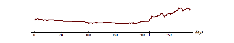
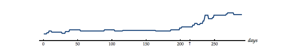
On 2 August 1990, the 214th day of that year, an event occurred in the Middle East that influenced the world-wide price of crude oil. The steep rise in price of a barrel of oil, shown in the middle panel of Figure 6.3, attests to this. An increase in the price of a liter of gasoline at retail distribution points would also follow from this. The question we pose is: what is the delay between a rise in prices at the wellhead and a rise in prices at the “pump”? How many days does it take before the price rises in the retail sale of gasoline?
To answer this we assume that the price of gasoline \(g[n]\) is a delayed version, that is function, of the price of crude oil \(c[n].\) But this cannot be expressed as simply \(g[n] = c[n - k].\) Between these two prices are complicated processes, some industrial and some marketplace. Nevertheless, one cannot help but being struck by the similarity of the top and bottom curves in Figure 6.3.
The cross-correlation between the two prices, under the assumption that the major effect is a time delay, can help us find the answer. Assuming that the system is a pure time delay, \(h[n] = \delta [n - k],\) and using Equation 6.17 gives:
| (6.37) |
$$\begin{array}{*{20}{l}}
{{\varphi _{cg}}[k]}&{ = {h^*}[k] \otimes {\varphi _{cc}}[k] = \delta [n - k] \otimes {\varphi _{cc}}[k]}\\
{\,\,\,}&{ = {\varphi _{cc}}[n - k]}
\end{array}$$
|
A simple substitution, \(m = n - k,\) allows us to rewrite this as
| (6.38) |
$${\varphi _{cg}}[n - m] = {\varphi _{cc}}[m]$$
|
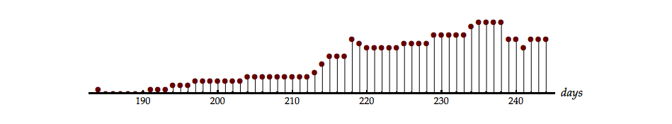
Applying Equation 6.32 to Equation 6.38 means that, given the model of a simple delay element, the time \(m = 0\) when the autocorrelation is a maximum is the same as the time \(m = n\) when the cross-correlation is a maximum. The cross-correlation is illustrated in Figure 6.4.
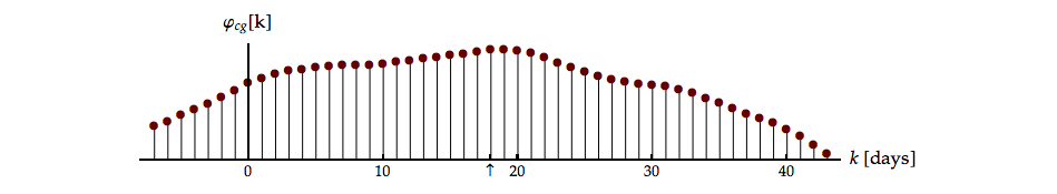
The time at which the maximum occurs is day 18. Our estimate for the time delay between the wellhead and the gasoline pump, in the midst of all the stochastic variations and the (over)simplification of the model, is 18 days.
Problems
Problem 6.1
The input to a discrete-time, LTI system is a stochastic signal, \(x[n].\) At each time step the output is \(+ \delta [n - k]\) with probability \(p\) or \(- \delta [n - k]\) with probability \(1 - p.\) Thus we can write:
where
The LTI system has \(h[n] = {\left( {\frac{1}{4}} \right)^n}u[n].\)
- Draw and label one possible stochastic signal \(x[n]\) from this random process.
- Draw and label \(y[n]\) the output signal corresponding to your choice of \(x[n].\)
- Determine \({m_y} = E\left\{ {y[n]} \right\}.\) Your answer should not contain any integrals or summations.
- Determine \({\varphi _{yy}}[k = 0] = {\left. {E\left\{ {y[n]\,{y^*}[n + k]} \right\}} \right|_{k = 0}}.\)
Problem 6.2
The impulse response of a discrete-time, LTI system is given by:
The input signal is a real, ergodic signal \(x[n]\) where:
The output signal of the LTI system is \(y[n].\)
- Determine \({m_y} = E\left\{ {y[n]} \right\}.\)
- Determine \({\varphi _{yy}}[k] = E\left\{ {y[n]\,{y^*}[n + k]} \right\}.\)
Problem 6.3
Discuss the following proposition:
The function \(f[k]\) given below cannot be the auto-correlation function of a stochastic signal.
Problem 6.4
When the discrete-time input signal \(x[n]\) is white noise with autocorrelation function \({\varphi _{xx}}[k] = \delta [k],\) the output signal from an LTI system is ergodic with power spectral density:
- Determine two possible causal, LTI filters \({H_1}\left( \Omega \right)\) and \({H_2}\left( \Omega \right)\) that could lead to this output power density spectrum.
- Given either of the filters, \({H_1}\left( \Omega \right)\) or \({H_2}\left( \Omega \right),\) from part (a), determine another, different noise signal \(q[n]\) that would yield the same \({S_{yy}}(\Omega )\) as given in part (a).
Problem 6.5
An ergodic process, \(x[n],\) is input to an LTI system with impulse response \(h[n]\) and Fourier transform \(H(\Omega ).\) The output is \(y[n].\) It is known that \(h[n = 0] \ne 0.\)
Discuss the following proposition:
If the mean of the input \(E\left\{ {x[n]} \right\} = {m_x} \ne 0\) then \(E\left\{ {y[n]} \right\} = {m_y} \ne 0.\)
Problem 6.6
Consider the following expression for a real, ergodic signal \(x[n]\):
| (6.39) |
$$E\left\{ {{{\left| {x[n] \pm x[n + k]} \right|}^2}} \right\} \geqslant 0$$
|
- Why is this expected value non-negative?
- Use this expression to prove Equation 6.32.
Laboratory Exercises
Laboratory Exercise 6.1
|
We now have the tools to analyze and discuss noise processes. We start with “white noise”. To start the exercise, click on the icon to the left. |
Laboratory Exercise 6.2
|
|
We continue the analysis and discussion of noise processes. We start with “binary noise”, a process that can be generated by flipping a coin. To start the exercise, click on the icon to the left. |
Laboratory Exercise 6.3
|
|
Can you estimate the parameters of real, ergodic noise processes based upon information from their number of samples N, their estimated autocorrelation function ${\varphi _{ \bullet \bullet }}[k]$, and/or their estimated power spectral density ${S_{ \bullet \bullet }}(\Omega ).$ To start the exercise, click on the icon to the left. |
Laboratory Exercise 6.4
|
When studying stochastic processes you not only have the mathematical tools we have presented, you also have your eyes and ears. To start the exercise, click on the icon to the left. |
Laboratory Exercise 6.5
|
|
We continue studying stochastic processes using the mathematical tools we have presented and your eyes and ears. To start the exercise, click on the icon to the left. |
Laboratory Exercise 6.6
|
|
We continue studying stochastic processes using the mathematical tools we have presented and your eyes and ears. To start the exercise, click on the icon to the left. |
Laboratory Exercise 6.7
|
|
Let us explore the effect that filtering has on various types of noise. As tools, we will use the noise signal itself, its amplitude distribution, its autocorrelation function, its power density spectrum, and your eyes and ears. To start the exercise, click on the icon to the left. |
Laboratory Exercise 6.8
|
|
How much information can you glean from the mathematical tools we have developed? To start the exercise, click on the icon to the left. |