The Wiener filter
In the previous chapter we showed that a desired effect, a maximized SNR, could be achieved by the suitable choice of a linear filter, a matched filter. We will now address a more difficult problem: the use of linear filters to estimate a stochastic signal in the presence of noise. We let \(x[n]\) be a stochastic, ergodic signal from a process with known statistics.
The restoration case: noise
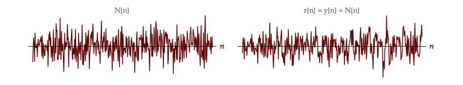
In the presence of noise and using a linear filter, we wish to produce an estimate of \(x[n]\) which we call \({x_e}[n].\) This is frequently termed signal restoration because we are attempting to restore a signal \(x[n]\) that has become damaged, corrupted, and/or noisy. We want the best estimate where the definition of “best” will be explained. We assume that \(x[n]\) is real as is the noise process \(N[n].\) The total signal \(r[n]\) composed of \(x[n]\) and \(N[n]\) is to be processed to produce the estimate \({x_e}[n]\) of the original \(x[n].\) The model is shown in Figure 10.1.
We start with:
| (10.1) |
$${x_e}[n] = \sum\limits_{m = - \infty }^{ + \infty } {r[n - m]} h[m]$$
|
and we define “best” in terms of a measure of the difference (error) between the “true” stochastic signal \(x[n]\) and the estimate \({x_e}[n].\)
Using the least mean-square error criterion
Specifically we look at the mean (expected) square error:
| (10.2) |
$$e = mean\text{-}squared\;error = E\left\{ {{{\left| {{x_e}[n] - x[n]} \right|}^2}} \right\}$$
|
and we propose to choose \(h[n]\) in order to minimize this error. We will need a basic result from least mean-square estimation theory and this can be found in Appendix I.
To determine a minimum, we look at:
| (10.3) |
$$\begin{array}{*{20}{l}}
{\frac{{\partial e}}{{\partial h}}}&{ = \frac{\partial }{{\partial h}}E\left\{ {{{\left| {{x_e}[n] - x[n]} \right|}^2}} \right\}}\\
{\,\,\,}&{ = \frac{\partial }{{\partial h}}E\left\{ {{{\left( {\sum\limits_{m = - \infty }^{ + \infty } {r[n - m]} h[m] - x[n]} \right)}^2}} \right\} = 0}
\end{array}$$
|
That is, we vary the filter to choose the one that gives the minimum mean-square error. Note that the restriction to real signals and systems ensures that we can replace the non-differentiable absolute value operation \({\left| \bullet \right|^2}\) with the differentiable operation \({\left( \bullet \right)^2}\) in Equation 10.3.
The equation above, of course, yields an extremum but it can be shown that this is a minimum; see Problem 10.1. The development of this approach follows those in the references Castleman1, Lee2, and Papoulis3.
Expressing the mean-square error
Based upon Appendix I, and starting from Equation 10.1 and Equation 10.2, we have:
| (10.4) |
$$\begin{array}{*{20}{l}}
e&{ = E\left\{ {{{\left( {{x_e} - x} \right)}^2}} \right\} = E\left\{ {{{\left( {{x_e}[n] - x[n]} \right)}^2}} \right\}}\\
{\,\,\,}&{ = E\left\{ {{{\left( {r[n] \otimes h[n] - x[n]} \right)}^2}} \right\}}\\
{\,\,\,}&{ = E\left\{ {{{\left( {\sum\limits_{k = - \infty }^{ + \infty } {r[n - k]h[k]} - x[n]} \right)}^2}} \right\}}
\end{array}$$
|
We might have expected that the left-hand side of Equation 10.4 would be \(e[n]\) instead of \(e.\) The expectation operation, \(E\left\{ \bullet \right\},\) combined with the assumption of ergodicity assures that the result \(e\) is independent of \(n.\)
We now apply the key result—orthogonality—from Equation 13.3 and rewrite this as:
| (10.5) |
$$0 = \frac{{de}}{{d{h_i}}} = \,2E\left\{ {\left( {\sum\limits_{k = - \infty }^{ + \infty } {r[n - k]h[k]} - x[n]} \right)r[n - i]} \right\}$$
|
Correlation returns
Rearranging this expression gives:
| (10.6) |
$$E\left\{ {x[n]r[n - i]} \right\} = E\left\{ {r[n - i]\sum\limits_{k = - \infty }^{ + \infty } {r[n - k]} h[k]} \right\}$$
|
The term on the left side of the equation is the cross-correlation function between \(x[n]\) and \(r[n].\) Because both signals are real, we have from Equation 5.5 and Equation 5.6:
| (10.7) |
$$E\left\{ {x[n]r[n - i]} \right\} = {\varphi _{xr}}[ - i] = \varphi _{rx}^*[i] = {\varphi _{rx}}[i]$$
|
Because the signal \(r[n - i]\) is not a function of \(k\) and the order of the operations of summation and expectation can—with all the usual caveats—be reversed, the term on the right side of the equation can be rewritten as:
| (10.8) |
$$\begin{array}{l}
E\left\{ {\sum\limits_{k = - \infty }^{ + \infty } {r[n - k]r[n - i]} h[k]} \right\} = \\
\,\,\,\,\,\,\,\,\,\,\,\,\,\,\,\sum\limits_{k = - \infty }^{ + \infty } {E\left\{ {r[n - k]r[n - i]} \right\}} h[k]
\end{array}$$
|
Again we have made use of Equation 4.13 which says that expectation as an operator distributes over sums.
The Wiener-Hopf equation
The result is an implicit expression for the optimum filter \(h[n]\):
| (10.9) |
$${\varphi _{rx}}[k] = \sum\limits_{m = - \infty }^{ + \infty } {{\varphi _{rr}}[k - m]} h[m] = {\varphi _{rr}}[k] \otimes h[k]$$
|
Note the way the variable names “\(m\)” and “\(k\)” are used in order to be consistent with earlier notation, for example, Equation 5.5 and Equation 5.6.
We distinguish between two cases of this famous equation, the Wiener-Hopf equation. The variable \(k\) represents the interval over which the process is observed. In the first case, \(k > 0\) and this represents the case of causal observations. That is, in principle, it is only possible to estimate \(x[n]\) from data that have already been gathered. The estimate \({x_e}[n]\) can only have a causal dependence on \(r[n]\) and the (causal) filter choice \(h[n].\) With this condition the solution of the Wiener-Hopf equation is extremely difficult, far beyond what we introduce here.
We will concentrate, instead, on the case \(- \infty \le k \le + \infty\) which admits a direct solution through application of Fourier techniques. While this case is somewhat less realistic for temporal signals (but not for spatial signals), it will enable us to develop some insights into the character of filters developed as solutions to the Wiener-Hopf equation. Such filters, independent of the conditions on \(k,\) are known as Wiener filters after a mathematical giant of the 20th century Prof. Norbert Wiener (1894-1964).
As seen from the Fourier domain
We start by taking the Fourier transform of both sides of Equation 10.9 to produce:
| (10.10) |
$${S_{rx}}(\Omega ) = {S_{rr}}(\Omega )H(\Omega )$$
|
The desired filter is, of course, \(H(\Omega )\) and this is given by:
| (10.11) |
$$H(\Omega ) = \frac{{{S_{rx}}(\Omega )}}{{{S_{rr}}(\Omega )}}$$
|
What is that least mean-square error?
Through a series of manipulations (following section 10.3 in Papoulis3), we show that the total minimum error \(e\) is:
| (10.12) |
$$e = \frac{1}{{2\pi }}\int\limits_{ - \pi }^{ + \pi } {\left( {{S_{xx}}(\Omega ) - {S_{rx}}(\Omega )H(\Omega )} \right)} d\Omega$$
|
We start with Equation 10.4 and using some algebra and the definition of the autocorrelation function we find:
| (10.13) |
$$\begin{array}{*{20}{l}}
e&{ = E\left\{ {{{\left( {{x_e}[n] - x[n]} \right)}^2}} \right\} }\\
{\,\,\,}&{ = E\left\{ {{x^2}[n]} \right\} + E\left\{ {x_e^2[n]} \right\} - 2E\left\{ {{x_e}[n]x[n]} \right\}}\\
{\,\,\,}&{ = {\varphi _{xx}}[0] + E\left\{ {x_e^2[n]} \right\} - 2E\left\{ {{x_e}[n]x[n]} \right\}}
\end{array}$$
|
Continuing with the use of Equation 10.1 this becomes a lengthy—somewhat inelegant— expression:
| (10.14) |
$$\begin{array}{*{20}{l}}
e&{ = {\varphi _{xx}}[0] + E\left\{ {x_e^2[n]} \right\} - 2E\left\{ {{x_e}[n]x[n]} \right\}}\\
{}&{ = {\varphi _{xx}}[0]\,\, + }\\
{}&{\,\,\,\,E\left\{ {\left( {\sum\limits_{m = - \infty }^{ + \infty } {r[n - m]} h[m]} \right)\left( {\sum\limits_{i = - \infty }^{ + \infty } {r[n - i]} h[i]} \right)} \right\}\,\, - }\\
{}&{\,\,\,\,\,2E\left\{ {\left( {\sum\limits_{m = - \infty }^{ + \infty } {r[n - m]} h[m]} \right)x[n]} \right\}}
\end{array}$$
|
Exchanging orders of expectation and summation, again, yields:
| (10.15) |
$$\begin{array}{*{20}{l}}
e&{ = {\varphi _{xx}}[0]\,\, + }\\
{\,\,\,}&{\,\,\,\,\,\,\sum\limits_{m = - \infty }^{ + \infty } {\left( {h[m]\sum\limits_{i = - \infty }^{ + \infty } {{\varphi _{rr}}[m - i]h[i]} } \right)} \,\, - }\\
{\,\,\,}&{\,\,\,\,\,\,2\left( {\sum\limits_{m = - \infty }^{ + \infty } {{\varphi _{rx}}[m]h[m]} } \right)}
\end{array}$$
|
In Equation 10.9 we determined an expression for the optimum filter, the filter that produces the minimum mean-square error. Substituting Equation 10.9 in Equation 10.15 yields:
| (10.16) |
$$e = {\varphi _{xx}}[0] - \sum\limits_{k = - \infty }^{ + \infty } {h[k]{\varphi _{rx}}[k]}$$
|
where, once again, we have replaced the dummy variable “\(m\)” with “\(k\)”. Using Equation 5.23 and Parseval’s Theorem, it is easy to see that Equation 10.16 is equivalent to Equation 10.12. See Problem 10.2.
Classic example, classic result
To proceed further we use one of the most common situations as an example. Let \(x[n]\) and \(N[n]\) be statistically independent and let \(N[n]\) have zero mean. Then:
| (10.17) |
$$\begin{array}{*{20}{l}}
{{\varphi _{nx}}[k]}&{ = E\left\{ {N[n]x[n + k]} \right\}}\\
{\,\,\,}&{ = E\left\{ {N[n]} \right\}E\left\{ {x[n + k]} \right\} = 0}
\end{array}$$
|
From the Wiener-Hopf equation, Equation 10.9, the desired quantities are \({\varphi _{rx}}[k]\) and \({\varphi _{rr}}[k]\):
| (10.18) |
$$\begin{array}{*{20}{l}}
{{\varphi _{rx}}[k]}&{ = E\left\{ {r[n]x[n + k]} \right\}}&{}&{}\\
{\,\,\,}&{ = E\left\{ {\left( {x[n] + N[n]} \right)x[n + k]} \right\}}&{}&{}\\
{\,\,\,}&{ = E\left\{ {x[n]x[n + k]} \right\} + E\left\{ {N[n]x[n + k]} \right\}}&{}&{}\\
{\,\,\,}&{ = {\varphi _{xx}}[k] + {\varphi _{nx}}[k]}&{}&{}
\end{array}$$
|
From Equation 10.17 we see that the second term is zero. Thus,
| (10.19) |
$${\varphi _{rx}}[k] = {\varphi _{xx}}[k]$$
|
or taking the Fourier transform of both sides,
| (10.20) |
$${S_{rx}}(\Omega ) = {S_{xx}}(\Omega )$$
|
Further, because \(r[n] = x[n] + N[n]\) and the noise is zero mean, we can show—see Problem 10.3—that:
| (10.21) |
$${S_{rr}}(\Omega ) = {S_{xx}}(\Omega ) + {S_{nn}}(\Omega )$$
|
Combining Equation 10.11, Equation 10.20, and Equation 10.21 results in:
| (10.22) |
$$H(\Omega ) = \frac{{{S_{xx}}(\Omega )}}{{{S_{xx}}(\Omega ) + {S_{nn}}(\Omega )}}$$
|
To better understand this result we look at two cases.
In the first case we consider those frequency regions where the signal strength (power) dominates the noise strength, that is, where
| (10.23) |
$${S_{xx}}(\Omega )\; > > \;{S_{nn}}(\Omega )$$
|
From our solution Equation 10.22 we see that this implies that \(H(\Omega ) = 1.\) In those frequency bands where the signal-to-noise ratio is high, the Wiener filter simply passes the input spectrum \(R(\Omega ) = {\mathscr{F}}\left\{ {r[n]} \right\}\) unchanged.
In the second case, we consider those frequency regions where the noise strength dominates the signal strength. We have:
| (10.24) |
$${S_{xx}}(\Omega )\; < < \;{S_{nn}}(\Omega )\,\,\,\,\,\, \Rightarrow \,\,\,\,\,\,H(\Omega ) = \frac{{{S_{xx}}(\Omega )}}{{{S_{nn}}(\Omega )}} \approx 0$$
|
The input spectrum \(R(\Omega )\) is almost completely attenuated by the Wiener filter.
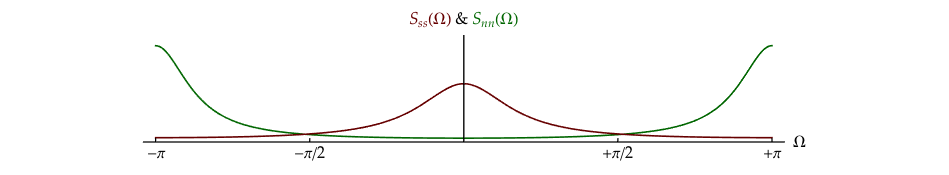
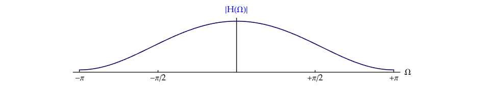
Figure 10.2 shows the linear filter spectrum generated by the signal and noise spectra given in an example in Chapter 8 and Figure 8.2.
The more general restoration case: noise & distortion
A more general formulation of the Wiener filter problem assumes not only a contamination of the input signal by random noise but also distortion of the input signal by a known linear filter \({h_o}[n].\) An example of this might be the blurred recording of an image due to camera motion where the noise source is the camera electronics. This situation is modeled in Figure 10.3.
Once again, we desire an \(h[n]\) that will minimize the expected square error between \(x[n]\) and \({x_e}[n].\)
We continue to assume real signals and systems, statistical independence of ergodic signal and ergodic noise, zero-mean signals, and zero-mean noise leading to \(E\left\{ {x[n]h[n + k]} \right\} = E\left\{ {x[n + k]h[n]} \right\} = 0.\)
Why we avoid the inverse filter
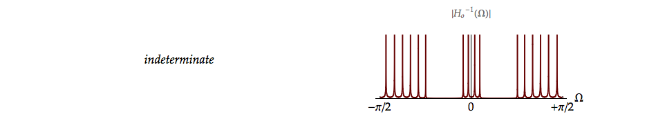
Our first temptation might be to use an inverse filter, \(H(\Omega ) = 1/{H_o}(\Omega )\) where \({H_o}(\Omega ) = {\mathscr{F}}\left\{ {{h_o}[n]} \right\}.\) The problem, however, lies in the behavior that the inverse filter will exhibit at those frequencies where \({H_o}(\Omega ) = 0.\)
At zeroes of the transfer function \({H_o}(\Omega ),\) the filter \(H(\Omega ) = 1/{H_o}(\Omega )\) will diverge. This will cause the noise to overwhelm the signal in precisely those frequency bands where the signal is weakest. The Wiener filter approach avoids this problem. An example of the problem caused by the inverse approach is shown in Figure 10.4.
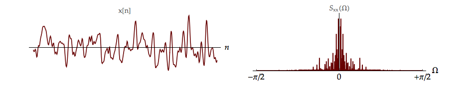
Example: Sound of (distorted) music
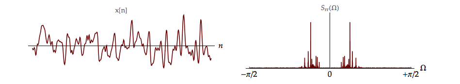
In the one-dimensional case illustrated4 in Figure 10.4, the signal is based upon a short section of Paganini’s violin concerto. The signal \(x[n]\) and its power spectrum \({S_{xx}}(\Omega )\) are shown.
It is interesting to consider if music can be treated as a stochastic signal. Certainly when Paganini wrote his Violin Concerto No. 1, every note is explicitly given as well as the manner that it should be played. Nevertheless, every performance of that music is different in unpredictable ways – the violinist, the violin, the temperature in the hall, the hall acoustics and so forth. Even with a digitally-recorded version, every listening experience differs due to room acoustics, position of the listener, electronic noise in the analog music reproduction, and environmental acoustical noise. We, therefore, use music as an example of a stochastic signal.
 ) to hear the original Paganini selection.
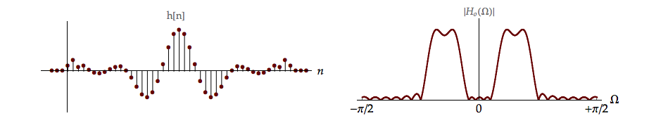
The signal is passed through a band-pass filter \({h_o}[n]\) with spectrum \({H_o}(\Omega )\) as shown in Figure 10.4.
) to hear a distorted version of the Paganini selection.
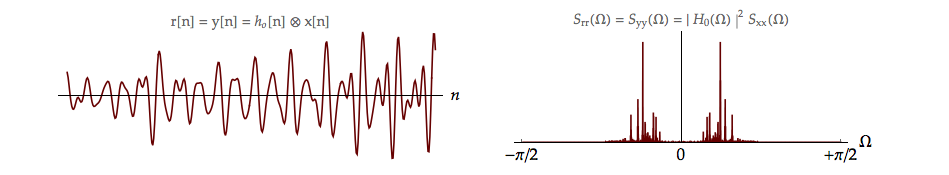
The output power spectrum of the filter is \({S_{yy}}(\Omega )\) and in the time domain the signal is \(y[n]\) as illustrated in Figure 10.3 and Figure 10.4. For the model shown in Figure 10.3, we assume (for now) that the noise is identically zero meaning \(r[n] = y[n].\) If the restoration filter is the inverse filter, \(H(\Omega ) = 1/{H_o}(\Omega )\) the zeroes in \({H_o}(\Omega )\) lead to infinities in the inverse and the output is indeterminate.
To make matters worse (and more realistic), we now look at what happens when the noise is not zero.
Example: Cleaning up our act
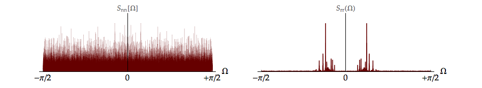
As shown in Figure 10.3, the filtered signal \(y[n]\) is now corrupted by noise which we will assume to be additive, white Gaussian noise. The effects in the time domain, the spectrum \(R(\Omega ),\) and the power spectral density \({S_{rr}}(\Omega )\) are shown in Figure 10.5.
Again, an inverse filter would lead to significant signal corruption as the zeroes of the \({H_o}(\Omega )\) which produce infinities in the inverse filter would now be multiplied by the non-zero spectral density values of the white noise. Adding noise exacerbates the problem of inverse filtering.
As “simple” inverse filtering is in many cases inadvisable, we, therefore, seek a filter technique that is “immune” to zeroes in \({H_o}(\Omega ).\)
Determining the Wiener filter
Once again we require \({\varphi _{rx}}[k]\) but
| (10.25) |
$$\begin{array}{*{20}{l}}
{{\varphi _{rx}}[k]}&{ = E\left\{ {r[n]x[n + k]} \right\}}&{}&{}\\
{\,\,\,}&{ = E\left\{ {\left( {y[n] + N[n]} \right)x[n + k]} \right\}}&{}&{}\\
{\,\,\,}&{ = E\left\{ {y[n]x[n + k]} \right\}}&{}&{}\\
{\,\,\,}&{ = {\varphi _{yx}}[k]}&{}&{}
\end{array}$$
|
This leads to (see Equation 6.22),
| (10.26) |
$${S_{rx}}(\Omega ) = {S_{yx}}(\Omega ) = H_0^*(\Omega ){S_{xx}}(\Omega )$$
|
Further,
| (10.27) |
$$\begin{array}{*{20}{l}}
{{\varphi _{rr}}[k]}&{ = E\left\{ {\left( {y[n] + N[n]} \right)\left( {y[n + k] + N[n + k]} \right)} \right\}}&{}&{}\\
{\,\,\,}&{ = {\varphi _{yy}}[k] + {\varphi _{nn}}[k]}&{}&{}
\end{array}$$
|
Taking the Fourier transform of both sides and using Equation 6.21 gives:
| (10.28) |
$$\begin{array}{*{20}{l}}
{{S_{rr}}(\Omega )}&{ = {S_{yy}}(\Omega ) + {S_{nn}}(\Omega )}\\
{\,\,\,}&{ = {{\left| {{H_0}(\Omega )} \right|}^2}{S_{xx}}(\Omega ) + {S_{nn}}(\Omega )}
\end{array}$$
|
The Wiener filter is once again defined through Equation 10.11 and, therefore,
| (10.29) |
$$H(\Omega ) = \frac{{H_0^*(\Omega ){S_{xx}}(\Omega )}}{{{{\left| {{H_0}(\Omega )} \right|}^2}{S_{xx}}(\Omega ) + {S_{nn}}(\Omega )}}$$
|
This is simply a general form of Equation 10.22 where a possible LTI distortion filter, \({{H_0}(\Omega )},\) has been taken into consideration. If there is no distortion filter, if \({H_o}(\Omega ) = 1,\) then Equation 10.29 reverts to Equation 10.22.
There are several useful ways to rewrite Equation 10.29. One of these is explored in Laboratory Exercise 10.5 and the reformulation is:
| (10.30) |
$$H(\Omega ) = \frac{{H_0^*(\Omega )}}{{{{\left| {{H_0}(\Omega )} \right|}^2} + \left( {\frac{{{S_{nn}}(\Omega )}}{{{S_{xx}}(\Omega )}}} \right)}}$$
|
For those frequencies where \({S_{xx}}(\Omega ) > > {S_{nn}}(\Omega ),\) the high-\(SNR\) frequency bands, the filter reduces to an inverse filter:
| (10.31) |
$$H(\Omega ) \approx \frac{{H_0^*(\Omega )}}{{{{\left| {{H_0}(\Omega )} \right|}^2}}} = \frac{1}{{{H_0}(\Omega )}} = H_0^{ - 1}(\Omega )$$
|
For those frequencies where \({S_{xx}}(\Omega ) < < {S_{nn}}(\Omega ),\) the low-\(SNR\) frequency bands, let
| (10.32) |
$$\frac{{{S_{nn}}(\Omega )}}{{{S_{xx}}(\Omega )}} \approx {N_0}\; > > \;1$$
|
Then the filter reduces to the matched filter solution as in Equation 9.12:
| (10.33) |
$$H(\Omega ) \approx \frac{1}{{{N_0}}}H_0^*(\Omega )$$
|
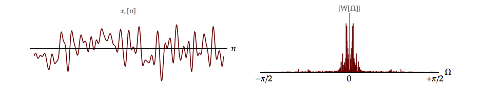
Finally, for those frequencies where \({H_o}(\Omega ) = 0,\) we see that \(H(\Omega ) = 0\) meaning no noise amplification. In Figure 10.6 we see an example of a Wiener filter designed to restore data after the effects of the bandpass filter used in Figure 10.4 and Figure 10.5.
 ) to hear a noisy, distorted version of the Paganini selection.
It is important to notice that the spectra \(\left\{ {{H_o}(\Omega ),{S_{xx}}(\Omega ),{S_{nn}}(\Omega )} \right\},\) that are required to implement the Wiener filter in Equation 10.29, are deterministic functions and not (stochastic) estimates. Such prior knowledge is rarely available so we are usually forced to estimate the spectra. Such estimation is the topic of the next chapter.
) to hear a Wiener-filter-restored version of the Paganini selection.
This example illustrates the power of Wiener filtering. The distortion and noise in \(r[n]\) are considerably—but not completely—reduced through the use of the Wiener filter.
Problems
Problem 10.1
Starting from Equation 13.3 show that the extremum is a minimum as opposed to a maximum or saddle point.
Problem 10.2
Consider two complex signals \(p[n]\) and \(q[n]\) with Fourier transforms \(P(\Omega )\) and \(Q(\Omega ).\)
| (10.34) |
$$\sum\limits_{k = - \infty }^{ + \infty } {q[k]{p^*}[k] = \frac{1}{{2\pi }}} \int\limits_{ - \pi }^{ + \pi } {Q(\Omega )} {P^*}(\Omega )d\Omega$$
|
Please note that this is the generalized form of Parseval’s Theorem. If \(q[n] = p[n],\) this then becomes the usual statement of the theorem.
- How does the result in part (a) change if both \(p[n]\) and \(q[n]\) are real signals?
- Using the result from part (b) show that Equation 10.16 can be rewritten as Equation 10.12.
Problem 10.3
Consider an ergodic, stochastic signal \(x[n]\) such as speech that has been corrupted by independent, additive ergodic noise \(N[n]\) so that the result is \(r[n] = x[n] + N[n].\)
- Determine an expression for \({\varphi _{rr}}[k]\) in terms of \({\varphi _{xx}}[k]\) (the autocorrelation function of the signal), \({\varphi _{NN}}[k]\) (the autocorrelation function of the noise), \({m_x}\) (the mean of \(x[n]\)), and \({m_N}\) (the mean of \(N[n]\)).
- What does \({\varphi _{rr}}[k]\) reduce to if the noise has zero-mean, that is, \({m_N} = 0?\)
- Determine the power spectral density of \(r[n]\) in terms of the power spectral densities of \(x[n]\) and \(N[n]\) assuming \({m_N} = 0.\)
Problem 10.4
The continuous-time music from Paganini used in the following sections Chapter 10, Chapter 10, and Chapter 10 was sampled at 44.1 kHz. In Figure 10.4, Figure 10.5, and Figure 10.6 the spectra are displayed from \(- \pi /2 \le \Omega \le + \pi /2\)
- What is the analog frequency range (in kHz) that is displayed in these figures?
- How can we justify displaying only these frequencies as opposed to the full spectra?
Note: In the following laboratory exercises involving audio signals, we will be freely switching between use of the discrete time frequency variable \(\Omega\) and the continuous frequency variable \(\omega = 2\pi f.\) The sampling rate remains 44.1 kHz.
Laboratory Exercises
Laboratory Exercise 10.1
|
A simple impulse has been corrupted by noise. Can the Wiener filter restore the signal and at what noise levels? Look and listen. To start the exercise, click on the icon to the left. |
Laboratory Exercise 10.2
 |
We explore the quality of the restoration of color images that can be achieved in the presence of significant amounts of noise. To start the exercise, click on the icon to the left. |
Laboratory Exercise 10.3
 |
We apply Wiener filtering to a two-dimensional signal, an image, that has first been distorted and then contaminated with noise. How faithful is the restored image? The mean-square error may have been minimized but is the image “pretty”? To start the exercise, click on the icon to the left. |
Laboratory Exercise 10.4
|
|
Images are acquired through cameras and all cameras have apertures. Can we restore an image that is distorted by an aperture effect and is “dirty” (noisy) as well? To start the exercise, click on the icon to the left. |
Laboratory Exercise 10.5
|
|
Using the Wiener-filter concept means having prior knowledge. What, for example, is the noise spectrum? If we make some assumptions and are prepared to justify these assumptions, perhaps we can simplify the problem with a “poor man’s Wiener filter”. To start the exercise, click on the icon to the left. |
-
Castleman, K. R. (1996). Digital Image Processing. Englewood Cliffs, New Jersey, Prentice-Hall ↩
-
Lee, Y. W. (1960). Statistical Theory of Communication. New York, John Wiley & Sons ↩
-
Papoulis, A. (1977). Signal Analysis. New York, McGraw-Hill ↩↩
-
The discrete-time signals x[n] and r[n] in this discussion are displayed as “continuous” curves because they contain thousands of samples and the standard display does not reproduce well. The spectra of the stochastic signals are displayed as line spectra because they are calculated from the Discrete Fourier Transform (DFT) using the FFT algorithm. Nevertheless, we continue to discuss discrete-time signals of the form \(f[n]\) and spectra as \(F(\Omega )\) as presented in the beginning of Chapter 3. ↩