The Matched Filter¶

How do you find a “needle in a haystack”? To start you have to know what a needle looks like. The “image” of a needle is a template and with one or more templates you then search through the haystack until a match is found. (Of course, other methods might be available like magnetic separation but here we focus on matching templates as opposed to haystack processing.)

Let the input to an LTI system be given by $x[n] + N[n]$ where $x[n]$ is a known signal (the “needle”) and for simplicity $x[n]$ is real. The real, impulse response of the system is $h[n]$ and the output $y[n]$ (the “haystack”) is:

(9.1)

$$y[n] = \left( {x[n] + N[n]} \right) \otimes h[n] = {y_x}[n] + {y_N}[n]$$

where ${y_x}[n]$ is the component of the output generated by the signal $x[n]$ and ${y_N}[n]$ is the component of the output generated by the real noise $N[n].$ We wish to determine a filter $h[n]$ such that, at a specified time $n = {n_0},$ the output signal-to-noise ratio (SNR) will be maximized. Why the SNR?

In communication theory¹, one learns that attempting to detect a signal always involves the possibility that an error will be made. Under a broad range of models it can be shown that maximizing the SNR leads to a minimization of the probability of error.

We cannot maximize the SNR by simply amplifying $y[n]$; both the signal and noise will be amplified and the SNR will remain the same. To search through the haystack $y[n]$ to detect the needle $x[n]$ we need filtering. We need the matched filter.

Setting up the problem¶

Assuming a zero-mean noise process and using a variation on Equation 8.2 to define the SNR at time $n = {n_0},$ we have:

(9.2)

$$S\tilde N{R_d} = \frac{S}{N} = \frac{{\left| {{y_x}[n = {n_0}]} \right|}}{{\sqrt {E\left\{ {{{\left| {{y_N}[n = {n_0}]} \right|}^2}} \right\}} }}$$

But from Equation 6.25:

(9.3)

$$\begin{array}{*{20}{l}} {E\left\{ {{{\left| {{y_n}[{n_0}]} \right|}^2}} \right\}}&{ = \frac{1}{{2\pi }}\int\limits_{ - \pi }^{ + \pi } {{{\left| {H( - \Omega )} \right|}^2}{S_{nn}}(\Omega )} d\Omega }\\ {\,\,\,}&{ = \frac{1}{{2\pi }}\int\limits_{ - \pi }^{ + \pi } {{{\left| {H(\Omega )} \right|}^2}{S_{nn}}(\Omega )} d\Omega } \end{array}$$

$H(\Omega )$ is the Fourier domain characterization of the filter to be found and we have used the fact that $h[n]$ is real to move from $H( - \Omega )$ to $H(\Omega ).$ Further, the $H(\Omega )$ that satisfies our requirement that the SNR be maximized will contain the parameter ${n_0}.$

Using Equation 9.1 and Equation 9.2 and remembering that in this specific discussion we are assuming that $x[n]$ as well as $h[n]$ is deterministic, we have:

(9.4)

$${y_x}[{n_0}] = \frac{1}{{2\pi }}\int\limits_{ - \pi }^{ + \pi } {X(\Omega )H(\Omega } ){e^{j\Omega {n_0}}}d\Omega$$

Using Cauchy-Schwartz¶

We now apply the Cauchy-Schwartz inequality²:

(9.5)

$${\left| {\int\limits_a^b {Z(\Omega )} W(\Omega )d\Omega } \right|^2} \le \left( {\int\limits_a^b {{{\left| {Z(\Omega )} \right|}^2}d\Omega } } \right)\left( {\int\limits_a^b {{{\left| {W(\Omega )} \right|}^2}d\Omega } } \right)$$

with equality if and only if $Z(\Omega ) = C\,{W^*}(\Omega )$ where $C$ is a real constant.

We rewrite Equation 9.4 as:

(9.6)

$${y_x}[{n_0}] = \frac{1}{{2\pi }}\int\limits_{ - \pi }^{ + \pi } {\frac{{X(\Omega )}}{{\sqrt {{S_{nn}}(\Omega )} }}H(\Omega } )\sqrt {{S_{nn}}(\Omega )} {e^{j\Omega {n_0}}}d\Omega$$

Using the inequality in Equation 9.5, we then have:

(9.7)

$${\left| {{y_x}[{n_0}]} \right|^2} \le \frac{1}{{2\pi }}\left( {\int\limits_{ - \pi }^{ + \pi } {\frac{{{{\left| {X(\Omega )} \right|}^2}}}{{{S_{nn}}(\Omega )}}} d\Omega } \right)\left( {\int\limits_{ - \pi }^{ + \pi } {{{\left| {H(\Omega )} \right|}^2}} {S_{nn}}(\Omega )d\Omega } \right)$$

Combining this result with our definition of $S\tilde NR$ from Equation 9.2 gives:

(9.8)

$${\left( {\frac{S}{N}} \right)^2} \le \int\limits_{ - \pi }^{ + \pi } {\frac{{{{\left| {X(\Omega )} \right|}^2}}}{{{S_{nn}}(\Omega )}}} d\Omega$$

This result is independent of our choice of $H(\Omega )$ and, further, fixes the largest signal-to-noise (SNR) ratio that can be attained. According to the Cauchy-Schwartz inequality, the maximum is reached if and only if:

(9.9)

$$\sqrt {{S_{nn}}(\Omega )} H(\Omega ) = C\frac{{{X^*}(\Omega )}}{{\sqrt {{S_{nn}}(\Omega )} }}{e^{ - j\Omega {n_0}}}$$

This can be rewritten to give the filter $H(\Omega )$ as:

(9.10)

$$H(\Omega ) = C\frac{{{X^*}(\Omega )}}{{{S_{nn}}(\Omega )}}{e^{ - j\Omega {n_0}}}$$

and an ${S\tilde N{R_d}}$ of:

(9.11)

$${\left( {S\tilde N{R_d}} \right)^2} = {\left( {\frac{S}{N}} \right)^2} = \int\limits_{ - \pi }^{ + \pi } {\frac{{{{\left| {X(\Omega )} \right|}^2}}}{{{S_{nn}}(\Omega )}}} d\Omega $$

The classic example¶

As an example, let ${S_{nn}}(\Omega ) = {N_o}$ that is, white noise of power density ${N_o}.$ From our solution for the matched filter, Equation 9.10, we have immediately:

(9.12)

$$H(\Omega ) = \frac{C}{{{N_0}}}{X^*}(\Omega ){e^{ - j\Omega {n_0}}}$$

Taking the inverse Fourier transform of both sides yields the impulse response:

(9.13)

$$h[n] = \frac{C}{{{N_0}}}x[{n_0} - n]$$

Example: Matching your filter¶

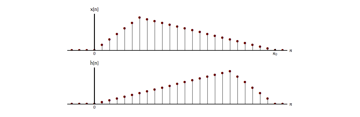
If $x[n]$ is as shown in Figure 9.1 below, then $h[n]$ will have the form that is also shown.

**Figure 9.1:** (*top*) The signal $x\lbrack n\rbrack $ and (*bottom*) the matched filter $h\lbrack n\rbrack = x\lbrack {n_0} - n\rbrack .$

The $S\tilde N{R_d}$ at time ${n_0}$ will be

(9.14)

$$\begin{array}{*{20}{l}} {S\tilde N{R_d}}&{ = \sqrt {\int\limits_{ - \pi }^{ + \pi } {\frac{{{{\left| {X(\Omega )} \right|}^2}}}{{{N_0}}}} d\Omega } = \sqrt {\frac{1}{{{N_0}}}\int\limits_{ - \pi }^{ + \pi } {{{\left| {X(\Omega )} \right|}^2}} d\Omega } }\\ {\,\,\,}&{ = \sqrt {\frac{{2\pi E}}{{{N_0}}}} } \end{array}$$

where $E$ is the energy in the signal $x[n].$

To further interpret this result we note that $h[n]$ is just a “flipped” version of $x[n]$ and this is what we call a matched filter. To explore this just a bit further, we note that ${y_x}[n]$ will be:

(9.15)

$${y_x}[n] = x[n] \otimes h[n] = x[n] \otimes \frac{C}{{{N_0}}}x[{n_0} - n]$$

The matched filter as an autocorrelation¶

Formally writing out the convolution gives:

(9.16)

$${y_x}[n] = \left( {\frac{C}{{{N_0}}}} \right)\sum\limits_{m = - \infty }^{ + \infty } {x[m]} x[m + n - {n_0}]$$

which, for real signals, is just the autocorrelation function of $x[n].$ That is:

(9.17)

$${y_x}[n] = \left( {\frac{C}{{{N_0}}}} \right){\varphi _{xx}}[n - {n_0}]$$

We have shown earlier, Equation 6.32, that the maximum of ${\varphi _{xx}}[k]$ occurs at $k = 0,$ that is, ${\varphi _{xx}}[k] \leqslant {\varphi _{xx}}[0].$ Translating this to the matched filter problem, we have that ${y_x}[n]$ is maximized (given the choice $h[n] \propto x[{n_0} - n]$) at $n = {n_0}.$

This cross-correlation between the two signals in Figure 9.1 is illustrated in Movie 9.1.

Movie 9.1: Cross-correlation of two signals. This involves first shifting one signal with respect to the other, then multiplying the signals point-by-point, and finally computing the “area” under their product.

It is important to remember that the cross-correlation depicted in Movie 9.1 is actually a convolution as described in Equation 9.15.

Performance in the presence of noise¶

As we saw in Figure 6.4, cross-correlation allows us to identify a peak, corresponding to a delay, in noisy (real) data. It is instructive to see how well this concept works at varying signal-to-noise ratios. We use the top signal in Figure 9.1 as a matched filter and a noisy version of the bottom signal in Figure 9.1 as the noisy input signal to the matched filter. We vary the SNR from 40 dB down to 0 dB according to the definition in Equation 8.3. The result is shown in Movie 9.2.

Movie 9.2: Output of the matched filter as the SNR varies from 40 dB down to 0 dB. Note the stability of the location of the peak position.

We see from this animation that the matched filter gives a robust method to estimate the peak position even at low values of the SNR.

Problems¶

Problem 9.1¶

The matched filter gives a robust method to find a signal in noise. We have seen this in Movie 9.2 and we will have the opportunity to experiment with this in the laboratory experiments in this chapter.

This suggests that we can perhaps use a matched filter to select one specific signal over other specific signals. Consider the four signals shown in Figure 9.2.

**Figure 9.2:** Four signals ${s_i}[n\rbrack,$ $\left\{ {i = 1,2,3,4} \right\}$ each of which is zero for $n < 0$ and $n > 7.$

Based upon Equation 9.15, determine and sketch the matched filter ${h_i}[n]$ for each of the four signals: ${s_i}[n],$ $\left\{ {i = 1,2,3,4} \right\}.$ Assume that $C = 1$ and ${N_o} = 1$ Watt/Hz.
Determine the output ${y_{ij}}[n]$ of each of the four matched filters $\left\{ {i = 1,2,3,4} \right\}$ for each of the four input signals $\left\{ {j = 1,2,3,4} \right\}.$ Hint: The use of various properties of convolution and correlation will save you a lot of work.
If each of the signals in part (b) is corrupted by additive, stationary Gaussian noise whose mean is zero and whose standard deviation is $\sigma,$ determine the mean of the output of each of the matched filters. The matched filters are not corrupted by noise.

Problem 9.2¶

The signals shown in Figure 9.2 are related to one another.

Describe, in words, any relationships you observe among the signals ${s_i}[n],$ $\left\{ {i = 1,2,3,4} \right\}.$

We want the four signals to convey information so we assign a meaning to each of the signals.

${s_1}[n]\,\,\, \Leftrightarrow \,\,\,{\rm{The\,Chicago\,Cubs\,will\,win\,the\,World\,Series}}$

${s_2}[n]\,\,\, \Leftrightarrow \,\,\,{\rm{The\,Chicago\,Cubs\,will\,win\,the\,NBA\, Championship}}$

${s_3}[n]\,\,\, \Leftrightarrow \,\,\,{\rm{The\,Chicago\,Cubs\,will\,win\,the\,Super\, Bowl}}$

${s_4}[n]\,\,\, \Leftrightarrow \,\,\,{\rm{The\,Chicago\,Cubs\,will\,not\,win\,the\,World\,Series}}$

We have tried to make the signals in Figure 9.2 as different from one another as possible in order to protect a message in the presence of additive noise. If the signals are different, then presumably it will still be possible to determine which message is being sent even when the signal is corrupted by noise. We measure the “difference” between two signals $x[n]$ and $y[n]$ as:

(9.18)

$${d_{xy}} = \sum\limits_{n = - \infty }^{ + \infty } {{{\left| {x[n] - y[n]} \right|}^2}}$$

Determine the difference ${d_{ij}}$ between each possible pair of the four signals ${s_i}[n],$ $\left\{ {i = 1,2,3,4} \right\}.$ Hint: Expanding the quadratic term before you start your computation can save you a lot of work.
According to our definition of difference, which signal pair is the most different?

The design of signals to facilitate communication in the presence of noise is described in communication theory and information theory. An excellent textbook for these topics is Wozencraft and Jacobs¹, in particular Chapter 4.

Laboratory Exercises¶

Laboratory Exercise 9.1¶

Movie 9.2 illustrated the stability of peak location in the presence of noise. In this exercise you will experiment with this result. Click on the icon to the left to start.

Laboratory Exercise 9.2¶

Finding a face in a crowd is similar to finding a needle in a haystack. You may have noticed this if you have ever tried to find Waldo (or Wally). Can matched filtering lend a hand or, better said, an eye? Click on the icon to the left to start.

Laboratory Exercise 9.3¶

Fourier analysis tells us that signals can be decomposed into weighted sums of sines and cosines. What happens if we use a sinusoid as a matched filter? To find out, click on the icon to the left.

Wozencraft, J. M. and I. M. Jacobs (1965). Principles of Communication Engineering. New York, John Wiley & Sons, Inc. ↩↩
An interpretation of the Cauchy-Schwartz inequality that makes it easier to understand is given by considering the inner product of two complex vectors a and b. This is given by the complex, scalar quantity a•b* = |a||b*|cos θ = |a||b|cos θ where θ is the angle between the two vectors, “*” denotes complex conjugation, and $\cos \theta = {\mathop{\rm Re}\nolimits} \{ {\bf{a}} \bullet {\bf{b}}\} /\left| {\bf{a}} \right|\left| {\bf{b}} \right|$ with Re the real part operator. The spectra $Z(\Omega )$ and $W(\Omega )$ can be considered as infinite-dimensional vectors. Because $\cos \theta$ is between $- 1$ and $+ 1,$ we have ${\left| {{\bf{a}} \bullet {\bf{b}}} \right|^2} \le {\left| {\bf{a}} \right|^2}{\left| {\bf{b}} \right|^2}$ which is the Cauchy-Schwartz inequality. The maximum value of the inner product is achieved when the two vectors are parallel, when $\theta = 0$ or $\theta = \pm \pi,$ in other words when ${\bf{a}} = C\,{\bf{b}}$ where $C$ is real. ↩