Introduction¶

In introductory studies of signals and systems we look at the class of input signals known as “deterministic” signals, signals where the value of the time function is known, by definition, for every time point $x[n]$. With the results derived in such studies we can calculate the outputs for linear, time-invariant (LTI) systems with impulse response $h[n]$ either through time domain convolution Equation 3.1:

(3.1)

$$ y[n] = x[n] \otimes h[n] \triangleq \sum\limits_{k = - \infty }^{ + \infty } x [k]h[n - k] $$

or through frequency domain multiplication:

(3.2)

$$ Y(\Omega)=X(\Omega)H(\Omega) $$

We assume an introductory level knowledge of signal processing and linear system theory. Such an introduction can be found in “Signals and Systems”¹.

The basics¶

The time domain $n$ and the frequency domain $\Omega$ representations of signals are related through the Fourier transform pair:

(3.3)

$$ \begin{aligned} X(\Omega)&=\sum_{n={-\infty}}^{+\infty}x[n]e^{{-j}\Omega n}\\ x[n]&=\frac{1}{2\pi}\int\limits_{-\pi}^{+\pi}X(\Omega)e^{+j\Omega n}d\Omega \end{aligned} $$

In shorthand notation, $X(\Omega)=\mathscr{F}\left\{x[n]\right\}$ and $x[n]=\mathscr{F}^{-1}\left\{X(\Omega)\right\}$ where $\mathscr{F}\left\{•\right\}$ is the Fourier transform operator. It is important that you are familiar with the computation and properties of Fourier transforms and inverse Fourier transforms and with convolution. The exercises in Problem 3.1 and Problem 3.3 review this material.

The first eight problems, in fact, are review problems in linear system theory and probability theory. If you find them difficult then you should review the textbooks in these disciplines. Several textbooks are listed below¹^,²^,³.

What is a random signal?¶

For an important class of input signals, however, the value of the signal at each time point is not known. Only very general properties of the input signal, referred to as averages, are available and it is with these averages that we must try to describe what happens at the output end of an LTI system. These signals are called stochastic or random signals and we can distinguish between two classes:

Random signals carrying information—e.g. speech, music, radio astronomy;
Random signals without information—noise.

We will describe both types of random signals in this iBook but, to do so, we must first develop some basic concepts concerning random signals and various averages of random signals. After that we will show how these concepts of stochastic signals can be used. We assume that you are familiar with basic probability theory but to review this material there is “Probability, Random Variables, and Stochastic Processes”² and the classical “Mathematical Methods of Statistics”³. The exercises in Problem 3.4 review this material.

We will develop several important themes including:

Signal-to-noise ratio (SNR) characterizations of systems;
Choosing linear filters for noise reduction;
Problems in estimation of Fourier spectra.

We begin with a simple model for generating a random signal in Example “Don’t bet on it”.

Example: Don’t bet on it¶

We throw a die once per second (discrete time) and the amplitude of the signal is the number of dots showing on the top die face. If at time $n=n_0$ the result is then:

(3.4)

$$x[n_0]=6\delta[n-n_0]$$

If the die is “fair” then the probability of die face #$i$ appearing on top, $p(i)$, will be the same for all faces and thus $p(1)=p(2)=\dots=p(6)=\frac{1}{6}$. This is just an example of the general requirements for a set of probabilities that could be associated with the six faces of a die.

(3.5)

$$\sum_{i=0}^{6}p(i)=1\text{ with }p(i)\geq 0 $$

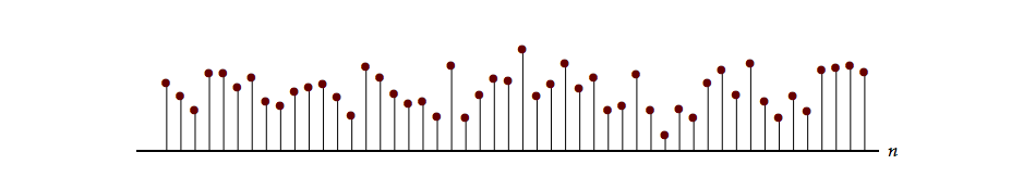
Over a period of time, that is a number of seconds, we can generate a random signal as shown in Figure 3.1.

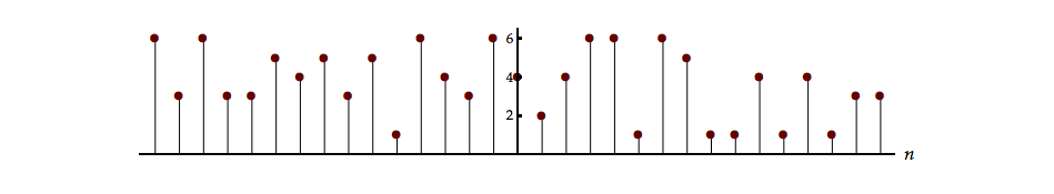
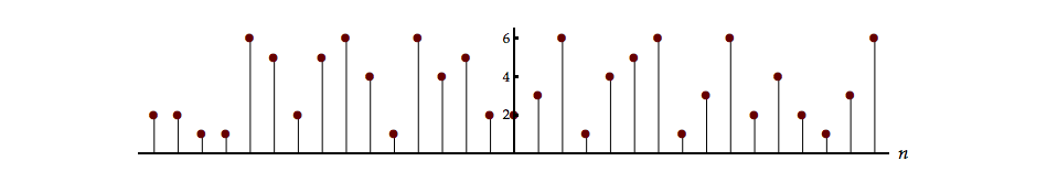
**Figure 3.1:** First realization of 31 random throws of a fair die.

This is just one realization of a random signal where the amplitudes are governed by a specific probability function. Performing the experiment again might lead to another realization as shown in Figure 3.2.

**Figure 3.2:** Second realization of 31 random throws of a fair die.

This concept will be illustrated, later, in Laboratory Exercise 4.1.

We can continue this procedure to generate an infinite number of realizations each governed by the same generating rule, throwing a fair die once per second and using the top face as a signal amplitude at that second. The possible collection of waveforms ($x_1[n]$, $x_2[n]$, $x_3[n]$, $x_4[n]$,…) together with the probability function for the amplitudes at time $n$ form a random process.

Instead of having the amplitudes governed by the throw of a die, we might find that the amplitudes are taken from the values on the continuous real line between ${-a}$ and $+a$ with probability density function:

(3.6)

$$p(\alpha)= \begin{cases} \frac{1}{2a} & \lvert\alpha\rvert\leq a\\ 0 & \lvert\alpha\rvert > a\\ \end{cases} $$

A graph of this probability function is given in Figure 3.3.

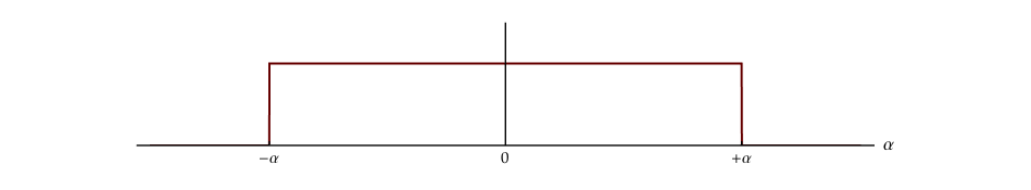
**Figure 3.3:** A uniform probability density function, $p(\alpha)$. All realizations between $-a$ and $+a$ are equally likely. The total probability (area under the curve) is 1.

It should be clear that at no time point will $\lvert x[n]\rvert > a.$ (Can you see why?) Thus $\vert x[n]\rvert \leq a.$ But the probability of the amplitude taking on the exact values $x[n]=+a$ or $x[n]={-a}$ is zero. (The proof of this is left to you; see Problem 3.5.)

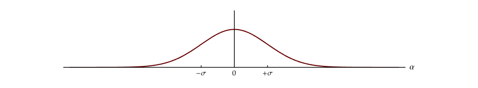
We might also consider that the amplitudes could be governed by the probability density function (pdf):

(3.7)

$$p(\alpha ) = \frac{1}{{\sigma \sqrt {2\pi } }}{e^{ - {\alpha ^2}/2{\sigma ^2}}}\quad {\kern 1pt} - \infty \leqslant \alpha \leqslant + \infty $$

This is perhaps the most well-known and well-studied continuous probability density function, the Gaussian (or normal) function. A graph of this probability function is given in Figure 3.4.

**Figure 3.4:** A Gaussian (normal) probability density function, $p(\alpha).$ Again, the total area under the curve is 1.

Examples of realizations from two random processes, one governed by a uniform probability density function and one by a Gaussian probability density function, are shown in Figure 3.5 and Figure 3.6. See Problem 3.6.

**Figure 3.5:** Example of samples from a Uniform density function ($\mu=1.0, \sigma=1/\sqrt{12}$)

**Figure 3.6:** Example of samples from a Gaussian density function ($\mu=1.0, \sigma=1/\sqrt{12}$)

Further, we could envision the situation where the random signal is generated by the composite rule from two distributions:

\[ \begin{aligned} n\text{ even }(n=\dots, -4, -2, 0, 2, \dots)\rightarrow p(x[n])&=\text{ throw die}\\ n\text{ odd }(n=\dots, -3, -1, 1, 3, \dots)\rightarrow p(x[n])&=\text{ choose from Gaussian} \end{aligned} \]

Of course, we can also talk about continuous-time random signals $x(t)$ where, for every instant $t,$ a rule is used to generate the value $x(t)$ leading to a random signal, a collection (ensemble) of realizations, and thus, together with the probability rule, a random process.

In our formulation of the random process based upon die throwing, we assumed that all throws were independent of each other, that is, independent events. Thus the outcome of throw n had no influence on the outcome of throw m and vice-versa. According to basic probability theory this means:

(3.8)

$$p(x[n]=i,x[m]=j)=p(x[n]=i)p(x[m]=j)\quad n\neq m;\quad i,j=1,\dots,6 $$

Two variables, $x$ and $y,$ are said to be statistically independent if $p_{x,y}(\alpha, \beta)=p_{x}(\alpha)p_{y}(\beta).$ Thus the die throwing described above forms a random process composed of statistically independent (SI) events. See Problem 3.7.

In summary and in preparing to do the following problems you should remember that this is neither an introductory textbook in signal processing nor an introductory textbook in probability theory. Should you have difficulties with these concepts, you should review one of the many textbooks available on these two subjects.

Problems¶

Problem 3.1¶

Compute the Fourier transform $X(\Omega)$ of the following signals:

$x[n]=\delta[n]=\begin{cases}1&n=0\\0&n\neq 0\end{cases}$
$x[n]=\delta[n-10]$
$x[n]=e^{{-j}\Omega_{0}n}$
$x[n]=\sin(\Omega_{0}n)$
$x[n]=e^{{-j}\Omega_{0}n}\sin(\Omega_{0}n)$
$x[n]=\left(\frac{1}{2}\right)^{-n}u[n]+2^{n}u[{-n}]-\delta[n]$
$x[n]=\begin{cases}1&\lvert n\rvert\leq N\\0&\lvert n\rvert >N\end{cases}$
$x[n]=\frac{\sin(n)}{\pi n}\otimes\frac{\sin(2n)}{\pi n}\text{ where}\otimes\text{ is convolution.}$

Problem 3.2¶

Compute the signal $x[n]$ described by the following Fourier transforms. Note that as all discrete-time Fourier transforms are periodic, $X(\Omega)=X(\Omega+2\pi),$ we describe the transform in the exercises below in the interval $- \pi \lt \Omega \le + \pi,$ the baseband.

$X(\Omega ) = \delta (\Omega )$
$X(\Omega)=\frac{1}{\left(1-\frac{1}{2}e^{{-j}\Omega}\right)\left(1-\frac{1}{3}e ^{{-j}\Omega}\right)}$
$X(\Omega)=\left(\frac{\sin(5\Omega/2)}{\sin(\Omega/2)}\right)^2$
$X(\Omega)=\frac{1}{2}(1+\cos^2(\Omega))$

Problem 3.3¶

For each of the examples given below $x[n]$ represents an input signal with Fourier transform $X(\Omega),$ $h[n]$ represents an impulse response of an LTI system with Fourier transform $H(\Omega),$ and $y[n]$ represents the output signal of the LTI system with Fourier transform $Y(\Omega).$

Given the description of the input and the LTI system below, determine the output $y[n].$

$x[n]=\delta[n]\qquad h[n]=\frac{\sin(\Omega_0n)}{(\pi n)}$
$x[n]=\delta[n-2]\qquad h[n]=\delta[n+3]$
$\begin{aligned}x[n]&=\alpha^n u[n]\qquad\lvert\alpha\rvert<1\\h[n]&=\beta^n u[n]\qquad\lvert\beta\rvert<1\end{aligned}\qquad \alpha \neq \beta$
$x[n]=e^{{-j}3n}\qquad h[n]=\frac{\sin(2n)}{(\pi n)}$
$\begin{aligned}x[n]&=\alpha^n u[n]\qquad\lvert\alpha\rvert<1\\h[n]&=\beta^n u[{-n}]\qquad\lvert\beta\rvert>1\end{aligned}\qquad \alpha \neq \beta$
$x[n]=\left(\frac{1}{7}\right)^n u[n]\qquad h[n]=\delta[n]-\frac{1}{7}\delta[n-1]$
$X(\Omega)=\left(\frac{\sin(5\Omega/2)}{\sin(\Omega/2)}\right)\qquad H(\Omega)=\left(\frac{\sin(3\Omega/2)}{\sin(\Omega/2)}\right)$
$\begin{aligned}x[n]&=\alpha^n u[{-n}]\qquad \lvert\alpha\rvert>1\\h[n]&=\beta^n u[{-n}]\qquad \lvert\beta\rvert>1\end{aligned}\qquad \alpha \neq \beta$

Problem 3.4¶

Each of the functions given below is intended to be a probability density function $p(x)$ in the continuous variable $x$ or a probability mass function $p(n)$ in the discrete variable $n.$ For each function determine the value of the constant $A,$ the value of the mean $\mu,$ and the value of the standard deviation $\sigma.$

$p(n)=A\delta(n-q)=\begin{cases}A&n=q\\0&n\neq q\end{cases}\quad n,q\in\mathbb{R}$
$p(x)=\begin{cases}Ae^{{-Bx}}&x\geq0\\0&x<0\end{cases}\quad B\in\mathbb{R}\text{ and }B>0$
$p(n)=A\frac{\lambda^{n}e^{{-\lambda}}}{n!}\qquad n\geq0\text{ and }n\in\mathbb{Z}$
$p(x)=\frac{A}{4+x^2}\qquad{-\infty}\leq x\leq{+\infty}$
$p(x)=\begin{cases}Axe^{-x^2/2}&x\geq 0\\0&x<0\end{cases}$

Problem 3.5¶

A uniform probability density function is defined in Equation 3.7.

What is the probability that the random variable $\alpha$ will lie in an interval of width $\Delta a$ where the interval is wholly contained in the region where $\left| \alpha \right| < a?$
What is the probability that $\alpha$ will lie in an interval of width $\Delta a$ where the interval is wholly contained in the region where $\left| \alpha \right| > a?$
Determine the mean $m_\alpha$ and the standard deviation $\sigma_\alpha$ of the random variable $\alpha$ for this uniform density function.

Problem 3.6¶

Determine mathematical formulas for the two probability density functions shown in Figure 3.5 and Figure 3.6. Your formulas should not involve any undefined parameters; all parameters should have a numerical value.

Problem 3.7¶

We throw two independent, fair dice as described in Example: Don’t bet on it producing the numbers $i$ and $j.$

Determine the probability that $i+j=11.$
Determine the probability mass function $p(r)$ where $r=\sqrt{i^2+j^2}$. That is, what are the values of $\left\{ p(\sqrt{2}),p(\sqrt{5}),p(\sqrt{8}),\dots,p(6\sqrt{2}) \right\}$?
Determine the mean value of $r,$ $m_r,$ and the standard deviation of $r,$ $\sigma_r.$

Problem 3.8¶

An even signal is defined by $x_e[n]=x_e[{-n}]$ and an odd signal is defined by $x_o[n]=-x_o[{-n}].$ Even and odd are symmetry properties. Answer each of the following:

Let $x[n]$ be an arbitrary signal. Determine the formulas that give the even part of $x[n]$ and the odd part of $x[n].$
Show that $x[n]$ can be represented by the sum of the even signal and the odd signal.
What is $x_o[n=0]?$
What is $\sum\limits_{n={-\infty}}^{+\infty}x_o[n]?$
What is $\sum\limits_{n={-\infty}}^{+\infty}x_e[n]x_o[n]?$
Express $\sum\limits_{n={-\infty}}^{+\infty}\lvert x[n]\rvert^2$ in terms of $x_e[n]$ and $x_o[n].$ Simplify your answer as much as possible.
Is $x_e[n]\cos(\Omega n)$ an even function of $n?$ What symmetry property is associated with the frequency variable $\Omega?$
Repeat the previous part for $x_e[n]\sin(\Omega n),$ $x_o[n]\cos(\Omega n)$ and $x_o[n]\sin(\Omega n).$
What symmetry properties can be associated with the Fourier transform $X(\Omega)$ of an arbitrary signal $x[n]?$ What properties can be expected if $x[n]$ is a real signal (as opposed to complex)?

Problem 3.9¶

The unit step function $u[n]$ has a Fourier transform given by:

\[U(\Omega)=\mathscr{F}\left\{u[n]\right\}=\left(\frac{1}{1-e^{{-j}\Omega}}\right) +\pi\delta(\Omega)\]

where, once again, the periodic spectrum is specified in the baseband $- \pi \lt \Omega \le + \pi.$ This will be discussed in a section in Chapter 5.

Determine the spectrum of the even part of $u[n]$ and the odd part of $u[n],$ that is, $U_e(\Omega)=\mathscr{F}\left\{u_e[n]\right\}$ and $U_o(\Omega)=\mathscr{F}\left\{u_o[n]\right\}.$
Does $U_o(\Omega)$ have the properties one should expect from the odd part of a real signal? Explain your answer.

Problem 3.10¶

This problem is in continuous time instead of discrete time but is, nevertheless, important because it has a link to probability theory. Full disclosure: We wrote this problem for the 2014 Dutch Physics Olympiad. Caveat emptor!

A linear, time-invariant system has impulse response $h(t),$ that is, when the input is $x(t)=\delta(t),$ the output is $y(t)=h(t).$ The output of this system can then be used as the input for one or more identical systems as shown below.

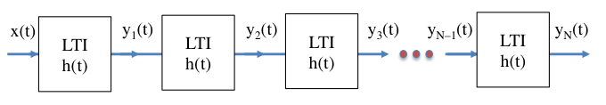
**Figure 3.7:** Concatenation of LTI systems.

The impulse response is given by:

\[ h(t)=\begin{cases}\frac{1}{2\sqrt{3}}&\lvert t\rvert\leq\sqrt{3}\\0&\lvert t\rvert>\sqrt{3}\end{cases} \]

Determine and sketch $H(\omega),$ the Fourier transform of $h(t).$ Your sketch should include labels and numerical values where possible.
Determine and sketch $y_1(t)$ and $y_2(t)$ when $x(t)=\delta(t).$ Again, your sketch should include labels and numerical values.
Sketch $y_3(t)$ and $y_{100}(t).$ You do not have to work out the analytical forms (unless you want to). And, yes, that is $N=100.$
Describe in words your result for $N=100.$ Be as precise as possible in your reasoning.

If we consider the class of signals that are everywhere non-negative, the center of a signal $y_c$ can be defined in the same way as the “center-of-gravity”. That is:

\[ y_c=\frac{\int\limits_{-\infty}^{+\infty}ty(t)dt}{\int\limits_{-\infty}^{+\infty}y(t)dt} \]

The root-mean-square width of a signal $y_{rms}$ can be similarly defined as:

\[ y_{rms}=\sqrt{\frac{\int\limits_{-\infty}^{+\infty}(t-y_c)^2y(t)dt}{\int\limits_{-\infty}^{+\infty}y(t)dt}} \]

Determine $y_c$ and $y_{rms}$ for $y_1(t),$ $y_2(t)$ and the general case $y_N(t).$ Reduce your answers to the simplest possible form.

The impulse response is now replaced by a new impulse response:

\[ h(t)= \begin{cases} \cos(5\pi t)&\lvert t\rvert\leq\sqrt{3}\\ 0&\lvert t\rvert>\sqrt{3} \end{cases} \]

Determine and sketch the new $H(\omega),$ the Fourier transform of the new $h(t).$ Your sketch should include labels and numerical values where possible.
Sketch $y_1(t)$ and $y_2(t)$ when $x(t)=\delta(t).$ Again, your sketch should include labels and numerical values. You do not have to give the analytical form for either signal.
Sketch $y_{100}(t).$ Again, you do not have to work out the analytical form (unless you want to). And, once again, that is $N=100.$

Oppenheim, A. V., A. S. Willsky and S. H. Nawab (1996). Signals and Systems. Upper Saddle River, New Jersey, Prentice-Hall ↩↩
Papoulis, A. and S. U. Pillai (2002). Probability, Random Variables, and Stochastic Processes. New York, McGraw-Hill ↩↩
Cramér, H. (1946). Mathematical Methods of Statistics. Princeton, New Jersey, Princeton University Press ↩↩