Characterization of Random Signals¶

Because it is impossible for us to specify what a random signal will be at any one instant, let alone for all $t$ or $n$, we have to settle for a description based upon average properties of the signal. There are a variety of definitions associated with the use of the word “average” (including “not very good”). In the context of this book we will focus on the concept as related to a number or property that is considered as representative of a collection of numbers such as those encountered in a signal.

Consider, for example, the flipping of a coin.

Example: Fair chance¶

We map Heads into +1 and Tails into –1 giving:

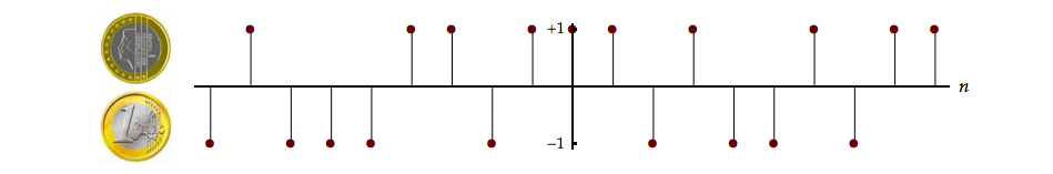
**Figure 4.1:** One realization of a coin-flipping experiment with Heads mapped to +1 and Tails mapped to –1

We might imagine computing the (arithmetic) average¹ over $2N + 1$ samples as:

(4.1)

$$ < x[n]{ > _{2N + 1}} = \frac{1}{{2N + 1}}\left( {\sum\limits_{n = - N}^{ + N} {x[n]} } \right) $$

In the above example:

For $N = 1 \to < x[n]{ > _3} = 1$

For $N = 2 \to < x[n]{ > _5} = 1/5$

For $N = 3 \to < x[n]{ > _7} = 3/7$

We “expect” for a “fair coin” that if $N$ is large then $< x[n]{ > _{2N + 1}} \approx 0$ because there will be just as many +1’s in the sum as –1’s.

Another way to compute the average is based upon knowledge of the distribution of $p(x[n])$ and is termed ensemble averaging. Instead of flipping one coin $N$ times we could flip $N$ coins once.

We then count the number of Heads $\left( {{n_H}} \right)$ and the number of Tails $\left( {{n_T} = N - {n_H}} \right)$. Our estimate of the probability of Heads would then be $p(H) = {n_H}/N$ and the probability of Tails as $p(T) = {n_T}/N = 1 - {n_H}/N$. Again for large values of $N$ and a “fair coin” we expect just as many Heads as Tails and this means $p(H) = p(T) = 1/2$. This method and stochastic signals associated with this method are explored in Laboratory Exercise 4.1.

By examining the probability of all the possible outcomes—in this case with a coin just two but in the case of a die six—we can develop a model for a probability distribution that describes the possible values of our random variable. And by associating numerical values to the variable, such as Heads $\rightarrow$ +1 and Tails $\rightarrow$ –1, we can compute averages.

Describing the ensemble average¶

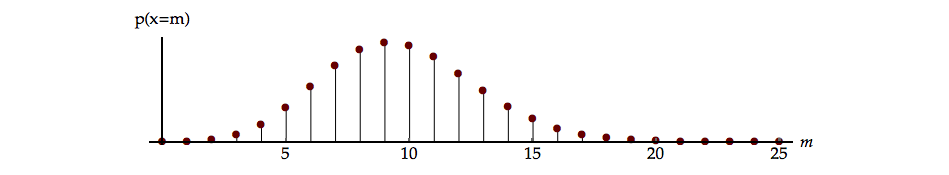
How do we do this? Returning to a statement above, we seek a number that is representative of a collection of random numbers. Let us assume that we have either a formal mathematical model of the random process that has generated the random numbers or we have collected sufficient data to have an excellent estimate of that probability distribution (or density) function. Either way we can depict—with confidence—the probability that the random variable $x$ can take on a specific value $m$ at time $n$. Such a probability distribution is shown in Figure 4.2.

**Figure 4.2:** Determining a representative number from a probability distribution. The distribution shown is a Poisson distribution.

If a single number is to characterize this distribution, a reasonable requirement is that the number provides a “balanced” description. From the domain of physics this has a specific meaning, the center-of-mass of a body with mass distribution, $m(\vec p).$ The classical distribution of mass, as we know, is a non-negative function of the position vector $\vec p.$ In that sense it is similar to a probability distribution. Finding the center-of-mass is equivalent to finding the position where the mass can be balanced. This is illustrated in Figure 4.3.

**Figure 4.3:** Determining a representative number from a mass (or probability) distribution. When the mass is distributed around the center-of-mass the object is balanced. When another position is chosen, unexpected and possibly unpleasant things can happen.

The mathematics associated with the calculation of the center-of-mass involve either $\int {\vec p} \,m(\vec p)d\vec p$ for a continuous (in space) distribution of mass or $\sum {{{\vec p}_i}} \,m({\vec p_i})$ for a discrete (in space) distribution of mass. See Sections I-18 and I-19 of Feynman².

It is but a short step to replace mass distribution (continuous or discrete) with a probability distribution (continuous or discrete) to define a number, the average, which is representative of a collection of random numbers. Indeed, this is the approach presented in Section 15.2 of Cramér³. This leads to a formal definition of averaging as:

(4.2)

$$ E \left\{ {x[n]} \right\} = \int\limits_{ - \infty }^{ + \infty } {x\,{p_{x[n]}}(x,n)dx = {m_{x[n]}}} $$

When the determination of an average is based upon the use of the probability distribution, it is referred to as an ensemble average⁴.

Here we take into consideration that the average or mean may depend on $n.$ (See, for instance, the even/odd mixed example above. In that example the probability distribution that is to be used in computing the average depends upon whether $n$ is even or odd.)

It may seem strange to see an integral in Equation 4.2 when we are talking about discrete-time signals. We should remember, however, that although time is discrete the values of the random variable need not be. They can, in principle, be complex numbers ${\Bbb C}$, real numbers ${\Bbb R}$, or integers ${\Bbb Z}$. The average value is computed over all possible values of the random variable of the amplitude $x$.

It is possible that a sum can be used instead of an integral. In Example: Average Experience, we see that the possible values of the random variable are indexed $i = 1, \ldots ,6$ in which case a sum is used. Another example is given in Problem 4.1 where $i = - \infty , \ldots ,0, \ldots , + \infty$ and a sum is again required. But in the most general formulation of averaging an integral is used⁵.

For many problems that occur—including those that we plan to focus on here—the random processes are stationary. This means that averages are in an equilibrium condition that is invariant to a shift in time. In a stationary die experiment we should obtain the same results (averages) whether the experiment is performed yesterday, today, or next year. For the mean value given above this would imply a value independent of the time origin:

(4.3)

$$ {m_{x[n]}} = {m_{x[n + k]}} = {m_{x[\ell ]}} = {m_x} $$

The mean value of the random process $x[n]$ at time $n$ is the same as at time $n + k.$ But this second time has its own “name” $\ell.$ This implies that the mean value is independent of time and is simply ${m_x},$ that is, stationary.

Example: Average experience¶

For our die experiment, where the number of possible outcomes can be indexed, we can use a version of the average based upon a sum:

(4.4)

$$ E\left\{ x \right\} = \sum\limits_{i = 1}^6 {{x_i}p({x_i})} = 1\left( {\frac{1}{6}} \right) + 2\left( {\frac{1}{6}} \right) + \ldots + 6\left( {\frac{1}{6}} \right) = \frac{7}{2} = {m_x} $$

Other averages¶

Other averages might, in general, be written as:

(4.5)

$$ Mean\;square = E\left\{ {{x^2}[n]} \right\} = \int\limits_{ - \infty }^{ + \infty } {{x^2}p(x[n])dx} $$

(4.6)

$$ E\left\{ {g\left( {x[n]} \right)} \right\} = \int\limits_{ - \infty }^{ + \infty } {g(x)p(x[n])dx} $$

To repeat, while $n$ is discrete, the random variable $x$ can have any value. For stationary processes these averages would reduce to:

(4.7)

$$ \begin{array}{l} E\left\{ {{x^2}} \right\} = \int\limits_{ - \infty }^{ + \infty } {{x^2}p(x)dx} \\ E\left\{ {g(x)} \right\} = \int\limits_{ - \infty }^{ + \infty } {g(x)p(x)dx} \end{array} $$

We apply these concepts to the example of throwing a die.

Example: Dice & money¶

(4.8)

$$ E\left\{ {{x^2}} \right\} = {1^2}\left( {\frac{1}{6}} \right) + {2^2}\left( {\frac{1}{6}} \right) + {3^2}\left( {\frac{1}{6}} \right) + \ldots + {6^2}\left( {\frac{1}{6}} \right) = 15\frac{1}{6} $$

If we use a function $g( \bullet )$ defined on the random variable $x$:

(4.9)

$$ g(x) = \left\{ {\begin{array}{*{20}{l}} { + 1}&{x\;{\rm{even}}\;2,\;4,\;6}\\ { - 1}&{x\;{\rm{odd}}\;1,\;3,\;5} \end{array}} \right. $$

Then the average value of this function of a random variable is:

(4.10)

$$ E\left\{ {g(x)} \right\} = 0 $$

We see through this choice of $g(x)$ that it is possible to use the die experiment to model the coin-flipping experiment. It is also important to realize that although we have chosen integer values for the random variable $x$ in Example: Fair chance, Example: Average experience and Example: Dice money, in general the variable can take on any complex value. The time index $n,$ of course, will remain discrete, that is, an integer.

We may also use two random variables $x[n]$ and $y[k]$ with an associated joint probability given by $p(x[n],y[k])$ and take the average:

(4.11)

$$ E\left\{ {x[n]y[k]} \right\} = \int\limits_{}^{} {\int\limits_{}^{} {x\,y\,p(x[n],y[k])dxdy} } $$

The more general function of the two random variables leads to an average:

(4.12)

$$ E\left\{ {g\left( {x[n],y[k]} \right)} \right\} = \int\limits_{}^{} {\int\limits_{}^{} {g(x,y)p(x[n],y[k])dxdy} } $$

We should remember that it is possible that $p(x[n],y[k])$ has a complicated behavior. The signal $x[n]$ may be based upon flipping a coin and the signal $y[n]$ may be based upon throwing a die. If these two types of events are independent, fair and stationary (caveat emptor!), then:

\[ p(x[n] = - 1,y[k] = 5) = p(x[n] = - 1)\,p(y[k] = 5) = \left( {\frac{1}{2}} \right)\left( {\frac{1}{6}} \right) = \frac{1}{{12}}\,. \]

While we have explicitly chosen two distinct time instances $n \ne k,$ this does not matter for calculation of the probability because we have also assumed that both signals are stationary. See Problem 4.2.

As we can infer from Figure 4.4, it is also possible that $y[k]$ is just the signal $x[n]$ at time $k.$ That is, if there is anything to be gained, there is nothing to prevent us from considering the case where $y[n] = x[n].$

**Figure 4.4:** Two samples $(x[n\rbrack,x[k\rbrack)$ can come from one realization of a random process. One sample is at time $n$ and the other at time $k.$

Properties of averaging¶

At this point, several well-known properties based upon linearity of averaging are useful to have available:

(4.13)

$$ E\left\{ {x[n] + y[n]} \right\} = E\left\{ {x[n]} \right\} + E\left\{ {y[n]} \right\} $$

(4.14)

$$ E\left\{ {ax[n]} \right\} = aE\left\{ {x[n]} \right\} $$

(4.15)

$$E\left\{ {x[n] + c} \right\} = E\left\{ {x[n]} \right\} + c$$

We will prove Equation 4.14 and leave the proofs of Equation 4.13 and Equation 4.15 for you at the end of this chapter. See Problem 4.3.

We start from Equation 4.2 and substitute $a\,x[n]$ where the constant $a$ is a deterministic—not random (!)—number:

(4.16)

$$\begin{array}{*{20}{l}} {E\left\{ {a\,x[n]} \right\}}&{ = \int\limits_{ - \infty }^{ + \infty } {a\,x\,p(x[n])dx} = a\int\limits_{ - \infty }^{ + \infty } {x\,p(x[n])dx} = a\,{m_{x[n]}}}\\ {}&{ = a\,E\left\{ {x[n]} \right\}} \end{array}$$

The first two properties, Equation 4.13 and Equation 4.14, indicate that the averaging operation is a linear operation. The average of a weighted sum of random variables, $x_1$ and $x_2,$ is the weighted sum of their averages, $E\left\{ {a\,{x_1} + b\,{x_2}} \right\} = a\,E\left\{ {{x_1}} \right\} + b\,E\left\{ {{x_2}} \right\}.$ As simple as each of these properties may seem, it is important that you understand how to prove each one and what each one means.

We have already looked at the averages mean and mean-square. Another important and therefore common average is the variance:

(4.17)

$$\begin{array}{*{20}{l}} {Variance\left\{ {x[n]} \right\}}&{ = \sigma _{x[n]}^2}\\ {}&{ = E\left\{ {{{\left( {x[n] - {m_{x[n]}}} \right)}^2}} \right\}}\\ {}&{ = E\left\{ {{x^2}[n]} \right\} - {{\left( {{m_{x[n]}}} \right)}^2}} \end{array}$$

which in the stationary form is given by:

(4.18)

$$Var\left( x \right) = \sigma _x^2 = E\left\{ {{{\left( {x[n] - {m_x}} \right)}^2}} \right\} = E\left\{ {{x^2}[n]} \right\} - m_x^2$$

We introduce here the notation $Var(x)$ to indicate the variance of the random variable $x.$ The term $\sigma,$ the positive square root of the variance, is called the standard deviation. Note that when the physical process generating $x[n]$ has a certain unit such as meters, then the standard deviation $\sigma$ has the same unit. The issue of units will be important later in this iBook when we discuss topics such as signal-to-noise ratio.

Correlation – the workhorse¶

These averages only describe what happens at a single time point of a random process even if the process is stationary. A more general and very useful average is the autocorrelation that describes the joint behavior of a random process at two points in time.

The motivation for examining this issue is that we would like to know if knowledge at one time point can help us predict or understand behavior at another time point. If a stochastic signal is increasing now, is it possible to predict that it might be decreasing 180 days from now?

Autocorrelation¶

In discrete time the definition of autocorrelation is:

(4.19)

$$\begin{array}{*{20}{l}} {{\varphi _{xx}}[n,k]}&{ = E\left\{ {x[n]\,{x^*}[k]} \right\} = E\left\{ {x[n]\,{x^*}[n + m]} \right\}}\\ {}&{ = {\varphi _{xx}}[n,n + m]} \end{array}$$

The procedure should be clear. We take the random variable at time $n$ and the random variable at time $k$ with their associated joint probability. We then ask: what is the expected value of their product?

The mechanics of correlations ¶

As an example we compute the expected value of the maximum temperature in Rotterdam, The Netherlands on 18 May 2013 multiplied by the maximum temperature in Rotterdam on 16 August 2013. We use data from the Royal Netherlands Meteorological Institute (KNMI). Their recordings for more than a century provide extensive information concerning what we frequently describe as “unpredictable weather”.

The maximum temperatures in Rotterdam for these two dates were 12.4 ºC and 26.4 ºC, respectively. But this is not enough. The result is not simply 327.36 ºC$^2,$ the product of the two numbers. We need to know the joint probability distribution of the two temperatures on those two specific days that are 90 days apart so that we can correctly compute the expected value. Estimating the joint probability distribution may not be easy.

As data collection in Rotterdam started in 1956, at the time of this writing only 60 years of data are available. Each year yields exactly one data pair $\left( {{T_{18 - May}},{T_{16 - Apr}}} \right).$ With a 0.1 ºC resolution and a potential temperature range of 20 ºC this means that approximately $200^2$ = 40,000 “cells” in a two-dimensional histogram are available. Any estimate based upon just 60 data points within 40,000 cells will be flawed. There is no underlying physical model (e.g. bivariate Gaussian) that we might wish to use. What should we do?

Our experience might suggest that within a one-week interval the temperature range is essentially the same with only statistical fluctuations. See “Predicting the natural climate – a case study” in Chapter 5.

But this would yield only 7 × 60 = 420 values for our 40,000 cells. Estimating the joint probability distribution $p\left( {{T_{18 - May}},{T_{16 - Apr}}} \right)$ is difficult.

Further, the maximum temperature values that we should expect will obviously be different if we choose instead 11 November 2013 and 9 February 2014 which are also 90 days apart. The maximum temperatures in Rotterdam for these last two days were 9.8 ºC and 7.6 ºC. The random process is not stationary.

It should also be clear that we could look at the temperature in Rotterdam on 18 May 2013 and the temperature at Amsterdam Airport (Schiphol) on that same day. These temperatures were 12.4 ºC and 12.5 ºC, respectively. The issue here is that the indices $n$ and $k$ need not be time; they could be spatial position. Once again we would need the joint probability distribution for these two temperature measurements at different spatial locations.

We emphasize that we have not invoked the assumption of stationarity, neither in time nor in space. The consequence of this is that we have two independent instances $n$ and $k.$ But we can always write $k$ as $n + m.$ (If $k = 10$ and $n = 7,$ then the difference between them is $m = + 3.$) The description of the probabilities and the averages derived with these probabilities will remain dependent on $(n,k)$ or $(n,n + m)$ and not simply the difference $m.$

Further, the use of the complex-conjugate notation $\left( {^ * } \right)$ as in Equation 4.19 implies that, unless otherwise indicated, we will be considering complex stochastic signals as well as real stochastic signals.

Auto-covariance¶

The auto-covariance is defined as:

(4.20)

$$\begin{array}{*{20}{l}} {{\gamma _{xx}}[n,k]}&{ = E\left\{ {\left( {x[n] - {m_{x[n]}}} \right){{\left( {x[k] - {m_{x[k]}}} \right)}^*}} \right\}}\\ {}&{ = {\varphi _{xx}}[n,k] - {m_{x[n]}}m_{x[k]}^*}\\ {}&{ = {\varphi _{xx}}[n,n + m] - {m_{x[n]}}m_{x[n + m]}^*} \end{array}$$

We leave it to you to derive the second line from the first line. See Problem 4.6.

Cross-correlation¶

Following on the idea introduced in Equation 4.11, that we can consider two signals $x[n]$ and $y[k],$ we also introduce the cross-correlation:

(4.21)

$$\begin{array}{*{20}{l}} {{\varphi _{xy}}[n,k]}&{ = E\left\{ {x[n]{y^*}[k]} \right\} = E\left\{ {x[n]{y^*}[n + m]} \right\}}\\ {}&{ = {\varphi _{xy}}[n,n + m]} \end{array}$$

Cross-covariance¶

Similarly, there is the cross-covariance for complex stochastic signals:

(4.22)

$$\begin{array}{*{20}{l}} {{\gamma _{xy}}[n,k]}&{ = E\left\{ {\left( {x[n] - {m_{x[n]}}} \right){{\left( {y[k] - {m_{y[k]}}} \right)}^*}} \right\}}\\ {}&{ = {\varphi _{xy}}[n,k] - {m_{x[n]}}m_{y[k]}^*}\\ {}&{ = {\varphi _{xy}}[n,n + m] - {m_{x[n]}}m_{y[n + m]}^*} \end{array}$$

We can immediately make the following observations: 1) In general ${\varphi _{xx}}[n,k],$ ${\varphi _{xy}}[n,k],$ ${\gamma _{xx}}[n,k]$ and ${\gamma _{xy}}[n,k]$ are all functions of two variables, and, 2) If $n = k,$ then

(4.23)

$$\begin{array}{l} {\varphi _{xx}}[n,k] = E\left\{ {{{\left| {x[n]} \right|}^2}} \right\}\\ {\gamma _{xx}}[n,k] = E\left\{ {{{\left| {x[n] - {m_{{x_n}}}} \right|}^2}} \right\} = \sigma _{{x_n}}^2\\ {\varphi _{xy}}[n,k] = E\left\{ {x[n]{y^*}[n]} \right\} \end{array}$$

If the process is stationary then the precise values of $n$ and $k$ are not important. Instead only $m = k - n,$ the time difference between them, is significant. Thus we have:

(4.24)

$$\begin{array}{l} {\varphi _{xx}}[n,k] = {\varphi _{xx}}[n,n + m] = E\left\{ {x[n]{x^*}[n + m]} \right\} = {\varphi _{xx}}[m]\\ {\varphi _{xy}}[n,k] = {\varphi _{xy}}[n,n + m] = E\left\{ {x[n]{y^*}[n + m]} \right\} = {\varphi _{xy}}[m] \end{array}$$

Notice that by definition we subtract the first index $n$ from the second $n + m$ to give $\left( {n + m} \right) - n = m.$

Example: Is that coin fair?¶

We return once again to the coin-flipping experiment for an example. We assume that the probability of Heads, $p(H),$ will be $p$ and the probability of Tails, $p(T),$ will be $1 – p.$ We associate with the occurrence of Heads a signal of +1 and with Tails a signal of –1. We note in passing that as $p(H)$ is not a function of time, this immediately implies that the random process is stationary. See also Problem 4.7.

We can now generate various realizations of this random process. Various averages, defined previously, can be determined as follows using the assumption that tosses of the coin occurring at differing instances of time will be statistically independent.

(4.25)

$${m_x} = ( + 1)(p)\; + \;( - 1)(1 - p) = 2p-1$$

(4.26)

$$E\left\{ {{x^2}} \right\} = {( + 1)^2}(p)\; + \;{( - 1)^2}(1 - p) = 1$$

(4.27)

$$\sigma _x^2 = 1 - {(2p - 1)^2} = 4p(1 - p)$$

(4.28)

$$\begin{array}{*{20}{l}} {{\varphi _{xx}}[k]}&{ = E\left\{ {x[n]{x^*}[n + k]} \right\}}\\ {}&{ = \left\{ {\begin{array}{*{20}{l}} {k = 0\;\; \Rightarrow }&{E\left\{ {{x^2}[n]} \right\} = 1}\\ {k \ne 0\;\; \Rightarrow }&{E\left\{ {x[n]} \right\} \bullet E\left\{ {x[n + k]} \right\} = m_x^2} \end{array}} \right.} \end{array}$$

Notice how the assumption of statistical independence of the coin flips allows us to write in the bottom line of Equation 4.28 that the average of the product equals the product of the averages.

For $p = 1/2$ (a fair coin where Heads is just as likely as Tails), we have ${m_x} = 0,$ $\sigma _x^2 = 1,$ and ${\varphi _{xx}}[k] = A\,\delta [k],$ the unit, discrete-time impulse. This last random signal $\left( {p = 1/2} \right)$ with independent and identically distributed signal values is pure noise and is termed white noise because the zero-mean, autocorrelation function is of the form ${\varphi _{xx}}[k] = A\,\delta [k]$ or, in the continuous-time case, ${\varphi _{xx}}(\tau ) = A\,\delta (\tau )$ where $A$ is a positive, real number. There are various definitions of white noise; we follow the description given in Section 2.5 of Porat⁶ and in Oppenheim⁷. Later in this iBook we will explain why this particular form of stochastic signal is termed “white” noise.

Describing the time average¶

As mentioned earlier it is also possible to compute the average of a signal as a time average:

(4.29)

$$< x[n] > \; = \mathop {\lim }\limits_{N \to \infty } \frac{1}{{2N + 1}}\sum\limits_{n = - N}^{ + N} {x[n]}$$

and the autocorrelation as:

(4.30)

$$< x[n]{x^*}[n + k] > \; = \mathop {\lim }\limits_{N \to \infty } \frac{1}{{2N + 1}}\sum\limits_{n = - N}^{ + N} {x[n]{x^*}[n + k]}$$

These two formulas both use a symmetric interval, $- N \leq n \leq + N,$ because we wish to capture the complete discrete-time series in our computation of an average: the past, the present and the future. For certain random processes, the following relations hold between the time average of a random process and the probabilistic average (ensemble average) of that same random process.

(4.31)

$${m_x} = E\left\{ {x[n]} \right\} = \; < x[n] >$$

(4.32)

$$\begin{array}{*{20}{l}} {{\varphi _{xx}}[k]}&{ = E\left\{ {x[n]{x^*}[n + k]} \right\}}\\ {}&{ = \; < x[n]{x^*}[n + k] > } \end{array}$$

Such a random process, where the time average equals the ensemble average, is known as an ergodic process⁸.

The ergodic process¶

One consequence of ergodicity is that it does not matter when computing an average—any average—whether one flips one coin $N$ times or $N$ coins once. From the definitions of time averages given above, it is clear that one condition that a random process must fulfill in order to be ergodic is that the process be stationary. All ergodic processes are stationary processes.

For an ergodic process the above result implies that, given a data record of finite length ${ x[n] },$ we can use finite-interval time averages to estimate the signal average and autocorrelation function even when the probability function is not explicitly known. The first step is to replace the limits in Equation 4.31 and Equation 4.32 with finite sums:

(4.33)

$${m_x} = \;{\kern 1pt} < x[n]{ > _{2N + 1}}\;{\kern 1pt} = \frac{1}{{2N + 1}}\sum\limits_{n = - N}^{ + N} {x[n]} $$

(4.34)

$$\begin{array}{*{20}{l}} {{\varphi _{xx}}[k]}&{ = \; < x[n]{x^*}[n + k]{ > _{2N + 1}}\;}\\ {}&{ = \frac{1}{{2N + 1}}\sum\limits_{n = - N}^{ + N} {x[n]{x^*}[n + k]} } \end{array}$$

In the following chapters we will make extensive use of the results from this chapter. In particular, in Chapter 5 we will further refine these equations.

It is important to note that while Equation 4.33 and Equation 4.34 are estimates of statistical properties of an ergodic process, this does not mean that they are good estimates. This issue will be discussed in greater detail in Chapter 11.

Problems¶

Problem 4.1¶

Consider the probability distribution described as follows:

\[p(i) = \left\{ {\begin{array}{*{20}{l}} {A{{\left( {\frac{1}{2}} \right)}^i}}&{i > 0}\\ 0&{i \le 0} \end{array}} \right.\]

where $i$ is an integer.

Determine the value of A.

Let the random variable $x$ associated with index i be given by ${2^{ - i}}.$

Determine the expected value $E\{ x\}.$

Problem 4.2¶

Schrödinger’s cat is back in the box. This time he is accompanied by two atoms each of a different isotope. The first isotope, ¹¹Be, has a half-life of ${t_{1/2}} = 13.81$s and its radioactive decay—a stochastic process—involves an electron $\left( {{\beta ^ - }} \right)$ emission. The second isotope, ¹⁰C, has a half-life of ${t_{1/2}} = 19.29$s and its radioactive decay involves a positron $\left( {{\beta ^ + }} \right)$ emission. Detectors inside the box can distinguish between these emitted particles.

If the ¹¹Be atom emits an electron, then poison gas will be released and the cat will immediately die. If the ¹⁰C isotope emits a positron, then the cat will be immediately released from the box and live.

What is the probability that within 20 seconds the cat will have been released and thus survived? Hint: The probability, $p(t),$ that an atom will decay either through electron or positron emission in the interval $0 \leqslant t \leqslant T$ seconds is given by:

\[P(0 \leqslant t \leqslant T) = 1 - {e^{ - T/\tau }}\]

where $\tau = {t_{1/2}}/\ln 2.$

Problem 4.3¶

Prove Equation 4.13 and Equation 4.15 .

Problem 4.4¶

In Equation 4.13, Equation 4.14, and Equation 4.15 we presented three important properties of averaging. The consequences when applied to the calculation of means should be obvious. There are, however, other averages and in this problem we look at the variance of a random variable.

Let $x$ be a random variable that has both a mean ${\mu _x}$ and a variance $\sigma _x^2.$ By this we mean that both ${\mu _x}$ and $\sigma _x^2$ exist and are finite. The random variable $y$ is related to $x$ by $y = a\,x + b$ where $a$ and $b$ are deterministic—not random—variables (or constants).

Determine the mean ${\mu _y}$ and variance $\sigma _y^2.$
What does this mean? Explain in words the meaning of the result for variance in relation to $b.$ How would this, for example, be reflected in a graph of the probability density function of $y$ relative to $x?$
If the coefficient-of-variation $C{V_x}$ of the random variable $x$ is given by $C{V_x} = {\sigma _x}/{\mu _x},$ where ${\mu _x} \ne 0,$ determine $C{V_y}$ in terms of the parameters given.

Problem 4.5¶

Let $x[n]$ be a sample from a random process $x$ with an underlying probability distribution that is stationary. The mean of the process is ${\mu _x}$ and the variance is $\sigma _x^2.$

The process $y$ is formed by $y[n] = x[n]\cos \left( {\Omega n} \right).$

What is the mean of process $y?$
What is the variance of process $y?$
Is process $y$ stationary?

Problem 4.6¶

Prove Equation 4.20.

Problem 4.7¶

We assume that when someone “flips” a coin that the $p(H) = p(T) = 1/2,$ what we call a “fair” coin. But with practice one could in principle learn to alter these probabilities. Fast Eddie has been practicing and he is learning. After $m$ practice sessions, his $p(H)$ is given by:

\[p(H) = \frac{1}{2}\left( {2 - {{\left( {\frac{1}{2}} \right)}^m}} \right)\]

Every time Heads ($H$) comes up, Eddie pays out $1; every time Tails ($T$) comes up, Eddie receives $1.

What is Eddie’s expected result with no training, that is, $m = 0?$
What is Eddie’s expected result after $m = 10$ training sessions?
Is Eddie working with a stationary random process?
Is Eddie “playing with a full deck”, that is, is he a rational player?

Problem 4.8¶

We are given a sample of an ergodic, continuous-time, white-noise random process, $x(t).$ We want to use samples of this continuous-time process to drive (as input to) a discrete-time system.

Discuss the following proposition and its consequences:

“There does not exist a finite sampling frequency, ${\omega _s} = 2\pi {f_s},$ that satisfies the Nyquist sampling theorem for x(t).”

Problem 4.9¶

In many discussions of random variables we encounter a phrase such as “without loss of generality we use the standardized (or normalized) random variable $z = \left( {x - {\mu _x}} \right)/{\sigma _x}$” where ${\mu _x}$ and ${\sigma _x}$ are the mean and standard deviation, respectively, of the random variable $x.$

Based upon what mathematical conditions is this statement justifiable?
What are the mean ${\mu _z}$ and the standard deviation ${\sigma _z}$ of the random variable $z$ if the conditions from part (a) have been satisfied?
Why is the expression “without loss of generality…” so frequently used?

Laboratory Exercises¶

Laboratory Exercise 4.1¶

Flipping (tossing) a coin is a well-known way to describe the generation of random events. If the coin is “fair” then we expect just as many occurrences of “Heads” as “Tails”. In this experiment we flip a coin N times with 1 ≤ N ≤ 81 and a probability of Heads where 0 ≤ p ≤ 1. The number of Heads n_H and the number of Tails n_T that result from N tosses of the coin will be displayed as a bar chart known as a histogram. You will also see a stochastic signal that is based upon your outcome and a lot of coins. To start the exercise, click on the icon to the left.

Laboratory Exercise 4.2¶

An N × N image consists of N² pixels. We can choose the grey-level brightness for each pixel from almost any distribution provided that the chosen value is real and non-negative. To start the exercise, click on the icon to the left.

There are other definitions of a “mean” than just the arithmetic mean. These are discussed briefly here. ↩
Feynman, R. P., R. B. Leighton and M. Sands (1963). The Feynman Lectures on Physics: Mainly Mechanics, Radiation, and Heat. Reading, Massachusetts, Addison-Wesley, Vol. I ↩
Cramér, H. (1946). Mathematical Methods of Statistics. Princeton, New Jersey, Princeton University Press ↩
For economy of notation, we will express ${{p_{x[n]}}(x,n)}$ (and similar forms) as $p(x[n])$. ↩
The sum formulation can be included within the integral formulation by describing the probability with the aid of impulse functions. In the die example, we would write the probability density function on the continuous variable $x$ as $p(x) = \sum\limits_{i = 1}^6 {\left( {\frac{1}{6}} \right)} \,\delta (x - i).$ ↩
Porat, B. (1994). Digital Processing of Random Signals: Theory & Methods. Englewood Cliffs, New Jersey, Prentice-Hall ↩
Oppenheim, A. V., R. W. Schafer and J. R. Buck (1999). Discrete-Time Signal Processing. Upper Saddle River, New Jersey, Prentice-Hall, Section 2.10 ↩
The word ergodic originated in the 20th century to describe the mathematical concept of a system or process with the property that, given sufficient time, it “visits” all points in a given space. Using the dictionary function of this iBook you can see the complete definition. ↩