Correlations and Spectra
Let \(x[n]\) and \(y[n]\) be two ergodic random processes. As stated in Chapter 4, this means that both processes are stationary.
Correlations: simple and complex
Based upon Equation 4.19 and Equation 4.21, we have that the autocorrelation function of the random process \(x\) and the cross-correlation function between processes \(x\) and \(y\) are:
| (5.1) |
$$\begin{array}{l}
{\varphi _{xx}}[k] = E\left\{ {x[n]{x^*}[n + k]} \right\}\\
{\varphi _{xy}}[k] = E\left\{ {x[n]{y^*}[n + k]} \right\}
\end{array}$$
|
While \(x\) and \(y\) are random processes, the auto- and cross-correlation functions are just ordinary, deterministic (not random) functions of the variable \(k.\) Why is that?
Because, like the mean \(\left( \mu \right)\) and standard deviation \(\left( \sigma \right)\) of familiar probability distributions, the correlations and covariances describe parameters—characteristics—of the probability distributions that generate random variables but are, themselves, not random.
The auto- and cross-covariance functions are given by:
| (5.2) |
$$\begin{array}{l}
{\gamma _{xx}}[k] = {\varphi _{xx}}[k] - {\left| {{m_x}} \right|^2}\\
{\gamma _{xy}}[k] = {\varphi _{xy}}[k] - {m_x}m_y^* \end{array}$$
|
By setting \(k = 0,\) we see that
| (5.3) |
$${\varphi _{xx}}[0] = E\left\{ {{{\left| {x[n]} \right|}^2}} \right\} = mean{\text -}square\;of\;process\; \ge 0$$
|
and
| (5.4) |
$${\gamma _{xx}}[0] = \sigma _x^2 \ge 0$$
|
Further, we have:
| (5.5) |
$$\begin{array}{l}
{\varphi _{xx}}[k] = \varphi _{xx}^*[ - k]\\
{\gamma _{xx}}[k] = \gamma _{xx}^*[ - k]
\end{array}$$
|
| (5.6) |
$$\begin{array}{l}
{\varphi _{xy}}[k] = \varphi _{yx}^*[ - k]\\
{\gamma _{xy}}[k] = \gamma _{yx}^*[ - k]
\end{array}$$
|
It is straightforward and, therefore, left to you to show in Problem 5.1 that Equation 5.5 and the second part of Equation 5.6 are correct. The proof of the first part of Equation 5.6 is given below.
We start from the second part of Equation 5.1 and replace \(n + k\) with \(m\):
which proves the first part of Equation 5.6 .
Example: Delayed effect
As a simple example we consider the case where \(y[n] = x[n - {n_o}],\) a delayed version of \(x[n].\) Then:
| (5.7) |
$$\begin{array}{*{20}{l}}
{{\varphi _{yy}}[k]}&{ = E\left\{ {y[n]\,{y^*}[n + k]} \right\}}\\
{}&{ = E\left\{ {x[n - {n_0}]\,{x^*}[n - {n_0} + k]} \right\}}\\
{}&{ = {\varphi _{xx}}[k]}
\end{array}$$
|
What does this mean? The conclusion associated with this example is that the autocorrelation of a time signal is independent of any time shift.
Correlations and memory
We would now like to consider what may happen to the correlation between \(x[n]\) and \(x[n + k]\) as \(k\) becomes larger. For many processes, as \(k \to \infty ,\) the value of the random signal at time \(n\) becomes less dependent upon the value at time \(n + k.\) A simple example might be that the weather today is similar to the weather yesterday but less similar to the weather of four weeks ago. As \(k \to \infty ,\) we have
| (5.8) |
$$\begin{array}{l}
\mathop {\lim }\limits_{k \to \infty } \left\{ {{\varphi _{xx}}[k] = E\left\{ {x[n]{x^*}[n + k]} \right\}} \right\}\\
\,\,\,\,\,\,\,\,\,\, = E\left\{ {x[n]} \right\}E\left\{ {{x^*}[n + k]} \right\} = {\left| {{m_x}} \right|^2}
\end{array}$$
|
This result frequently holds as well for the cross-correlation giving:
| (5.9) |
$$\mathop {\lim }\limits_{k \to \infty } {\varphi _{xy}}[k] = {m_x}m_y^*$$
|
Finally these two results may be used to show that for many important cases:
| (5.10) |
$$\begin{array}{l}
\mathop {\lim }\limits_{k \to \infty } {\gamma _{xx}}[k] = 0\\
\mathop {\lim }\limits_{k \to \infty } {\gamma _{xy}}[k] = 0
\end{array}$$
|
As \(k \to \infty ,\) correlations and covariances can exhibit a form of memory loss, of forgetting their relation to earlier values.
These results provide us with tools that can help us estimate the long term correlation and variation of one or more random processes. We have specifically stated “many processes” but not “all processes”. See Problem 5.2 to explore this.
The mechanics of correlations - redux
An issue that we have avoided until now is: how do we actually calculate the autocorrelation or cross-correlation of a random signal? According to Equation 4.24, we need to know the joint probability distributions at two points \(n\) and \(n + m.\) Under the assumption of stationarity this reduces from \(\varphi [n,n + m]\) to \(\varphi [m].\) But given an actual random process such as air pressure, internet traffic, or radioactive emissions, we almost never know the joint probability distribution including the values of all of its parameters. Under the assumption of ergodicity, as described in Chapter 4 here and here, an alternative method is available to us.
When considering the autocorrelation function, for example, instead of using Equation 4.24 we can use Equation 4.30. Both of these equations are repeated below in Equation 5.11 and they illustrate that for ergodic processes ensemble averages can be exchanged for time averages.
| (5.11) |
$$\begin{array}{*{20}{l}}
{{\varphi _{xx}}[k]}&{ = E\left\{ {x[n]\,{x^*}[n + k]} \right\}}\\
{}&{ = \; < x[n]\,{x^*}[n + k] > }\\
{}&{ = \mathop {\lim }\limits_{N \to \infty } \frac{1}{{2N + 1}}\sum\limits_{n = - N}^{ + N} {x[n]\,{x^*}[n + k]} }
\end{array}$$
|
Even with this reformulation there remains a problem. We never have an infinite amount of recorded data; \(N\) never goes to infinity. This brings us instead to Equation 4.34 where a finite amount of data is used to estimate a correlation function. This means that we can use the following formulation.
| (5.12) |
$$\begin{array}{l}
{\varphi _{xx}}[k] = \;\frac{1}{{2N + 1}}\sum\limits_{n = - N}^{ + N} {x[n]\,{x^*}[n + k]} \\
{\varphi _{xy}}[k] = \;\frac{1}{{2N + 1}}\sum\limits_{n = - N}^{ + N} {x[n]\,{y^*}[n + k]}
\end{array}$$
|
As the term \(1/\left( {2N + 1} \right)\) is only a scale factor—albeit an important one when comparing estimates of correlation functions based upon data sets of different lengths—we further simplify this to:
| (5.13) |
$$\begin{array}{l}
{\varphi _{xx}}[k] = \;\sum\limits_{n = - N}^{ + N} {x[n]\,{x^*}[n + k]} \\
{\varphi _{xy}}[k] = \;\sum\limits_{n = - N}^{ + N} {x[n]\,{y^*}[n + k]}
\end{array}$$
|
The formulas for calculating the autocorrelation and crosscorrelation of stochastic signals are now similar to the ones for deterministic signals Oppenheim1.
To summarize, if the processes we are studying are ergodic, we use finite data sets to calculate correlation functions (and means and covariance functions). Papoulis2 stated this in a most succinct way:
This, of course, holds for discrete-time ergodic processes as well.
Fourier description of correlation functions
We now look at the Fourier transform of the autocorrelation function for the complex ergodic random process \(x[n].\) We should remember that \({\varphi _{xx}}[k]\) is not a random process. The Fourier transform of the autocorrelation function—if it exists—is called the power spectrum (or power density spectrum) of the random process. This name will be explained later.
Existence of the Fourier transform is not a trivial matter. A random process \(x[n]\) might be ergodic but it need not be absolutely integrable, a condition for the existence of its Fourier spectrum; see Section 5.1.3 of Oppenheim1. The same holds for the autocorrelation function associated with \(x[n].\)
A digression
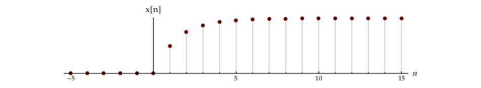
Ignoring the issue of convergence can lead to surprising results. Consider, for example, the deterministic signal given by:
| (5.14) |
$$x[n] = \left( {1 - {{\left( {\frac{1}{2}} \right)}^n}} \right)u[n]$$
|
This signal is depicted in Figure 5.1.
As mentioned before, the autocorrelation of a deterministic signal is defined by Oppenheim1:
| (5.15) |
$${\varphi _{xx}}[k] = \sum\limits_{n = - \infty }^{ + \infty } {x[n]{x^*}[n + k]}$$
|
Substituting the specific signal Equation 5.14 into Equation 5.15 gives:
| (5.16) |
$${\varphi _{xx}}[k] = \sum\limits_{n = - \infty }^{ + \infty } {\left( {1 - {{\left( {\frac{1}{2}} \right)}^n}} \right)\left( {1 - {{\left( {\frac{1}{2}} \right)}^{n + k}}} \right)u[n]u[n + k]}$$
|
The two step functions \(u[n]\) and \(u[n + k]\) both “start”—go from 0 to 1—at some finite time and then remain at 1 as \(n\) increases. Their product starts at \(\max \left( {0, - k} \right).\) If \(k \ge 0,\) then the start time of the product is \(n = 0.\) If \(k < 0,\) then the start time of the product is \(n = - k.\) From Equation 5.5 we know that the autocorrelation of a signal, whether it is deterministic or stochastic, is an even function. This means we only have to evaluate Equation 5.16 for \(k \ge 0.\) The rest will follow from the even symmetry.
Multiplying the various terms in Equation 5.16, the first of which yields \(\sum\nolimits_n 1,\) it should be obvious that this sum diverges.
To study the behavior of Equation 5.16 we introduce a window function, \(w[n]\):
| (5.17) |
$$w[n] = \left\{ {\begin{array}{*{20}{c}}
1&{\left| n \right| \le N}\\
0&{\left| n \right| > N}
\end{array}} \right.$$
|
such that \(x[n]\) is replaced by \(x[n]\,w[n].\) Eventually we will let \(N \to \infty.\) The autocorrelation is then rewritten for \(k \ge 0\) as:
| (5.18) |
$$\begin{array}{l}
{\varphi _{xx}}[k] = \sum\limits_{n = - \infty }^\infty {\left( {1 - {{\left( {\frac{1}{2}} \right)}^n}} \right)w[n]\left( {1 - {{\left( {\frac{1}{2}} \right)}^{n + k}}} \right)} w[n + k]\\
\,\,\,\,\,\, = \sum\limits_{n = 0}^{N - k} {\left( {1 - {{\left( {\frac{1}{2}} \right)}^n}} \right)\left( {1 - {{\left( {\frac{1}{2}} \right)}^{n + k}}} \right)}
\end{array}$$
|
Notice how the limits on the sum have changed. Four terms are involved in this sum, the last three of which are “well-behaved”; they converge as \(N \to \infty.\) The result including the even symmetry is:
| (5.19) |
$${\varphi _{xx}}[k] = \left( {\mathop {\lim }\limits_{N \to \infty } N} \right) - \left| k \right| - \left( {\frac{2}{3}} \right){\left( {\frac{1}{2}} \right)^{\left| k \right|}} - 1$$
|
The result is shown in Figure 5.2.

The seemingly simple deterministic signal \(x[n]\)—a signal which is not a pathological oddity but, in fact, describes a variety of common, physical processes—does not have a simple autocorrelation function. Why is this?
In the time domain it is obvious from Figure 5.1 that \(x[n]\) is summable in neither the absolute sense (L1–norm) nor the quadratic sense (L2–norm). Thus the sum in Equation 5.16 is, formally, not possible.
The Fourier transform of \(x[n]\) also provides insight into the problem. The spectrum \(X\left( \Omega \right)\) is given by:
| (5.20) |
$$\begin{array}{*{20}{l}}
{X(\Omega )}&{ = \sum\limits_{n = - \infty }^{ + \infty } {x[n]{e^{ - j\Omega n}}} = \sum\limits_{n = - \infty }^{ + \infty } {\left( {1 - {{\left( {\frac{1}{2}} \right)}^n}} \right)u[n]{e^{ - j\Omega n}}} }\\
{}&{ = \sum\limits_{n = - \infty }^{ + \infty } {u[n]{e^{ - j\Omega n}}} - \sum\limits_{n = - \infty }^{ + \infty } {{{\left( {\frac{1}{2}} \right)}^n}u[n]{e^{ - j\Omega n}}} }\\
{}&{ = {\rm{ }}{\mathscr{F}}\left\{ {u[n]} \right\} - \sum\limits_{n = 0}^{ + \infty } {{{\left( {\frac{1}{2}} \right)}^n}{e^{ - j\Omega n}}} }\\
{}&{ = {\rm{ }}{\mathscr{F}}\left\{ {u[n]} \right\} - \left( {\frac{1}{{1 - \frac{1}{2}{e^{ - j\Omega }}}}} \right)}
\end{array}$$
|
The difficulty originates in the first term, the Fourier transform of a unit step function. This transform is known Oppenheim1 and Oppenheim3 and is given in the baseband \(- \pi \lt \Omega \le + \pi\) by:
| (5.21) |
$${\mathscr{F}}\left\{ {u[n]} \right\} = \left( {\frac{1}{{1 - {e^{ - j\Omega }}}}} \right) + \pi \,\delta (\Omega )$$
|
This spectrum of a discrete-time signal is, of course, periodic and is specified in Equation 5.21 in the baseband frequency range, \(- \pi \lt \Omega \le + \pi.\) Both terms in Equation 5.21 diverge for \(\Omega = 0\) and the behavior of \({\left| {X(\Omega )} \right|^2}\)—whose relevance will be discussed later—becomes intractable.
This may all seem like “much ado about nothing” but that is not the case. We will make extensive use of the Fourier representation of stochastic signals as in the example in Chapter 5 and, as we shall see in Chapter 7, the divergence “problem” shown above may provide insights into the behavior of physical processes.
The power density spectrum and its properties
When the autocorrelation function exists, the power density spectrum is given by:
| (5.22) |
$${S_{xx}}(\Omega ) = {\mathscr{F}}\left\{ {{\varphi _{xx}}[k]} \right\} = \sum\limits_{k = - \infty }^{ + \infty } {{\varphi _{xx}}[k]{e^{ - j\Omega k}}}$$
|
Standard Fourier theory gives the inverse transform as:
| (5.23) |
$${\varphi _{xx}}[k] = {\mathscr{F}^{ - 1}}\left\{ {{S_{xx}}(\Omega )} \right\} = \frac{1}{{2\pi }}\int\limits_{ - \pi }^{ + \pi } {{S_{xx}}(\Omega )} {e^{ + j\Omega k}}d\Omega$$
|
Note that \({S_{xx}}(\Omega )\) does not require the convergence condition to perform the inverse transform in Equation 5.23 as it is periodic in the frequency domain and the integral involves the interval from \(- \pi\) to \(+ \pi.\) When the convergence conditions in the time-domain are satisfied then we can describe and use the Fourier transform pair \(\left\{ {{\varphi _{xx}}[k],{S_{xx}}(\Omega )} \right\}\) as shown in the Wiener-Khinchin theorem.
If we now substitute Equation 5.13 into Equation 5.22, the power density spectrum of the ergodic signal \(x[n]\) can be written as:
| (5.24) |
$$\begin{array}{*{20}{l}}
{{S_{xx}}(\Omega )}&{ = \sum\limits_{k = - \infty }^{ + \infty } {{\varphi _{xx}}[k]{e^{ - j\Omega k}}} }\\
{}&{ = \;\sum\limits_k {\left( {\sum\limits_n {x[n]{x^*}[n + k]} } \right)} {e^{ - j\Omega k}}}\\
{}&{ = \;\sum\limits_n {x[n]\sum\limits_k {{x^*}[n + k]{e^{ - j\Omega k}}} } }\\
{}&{ = \sum\limits_n {x[n]{e^{j\Omega n}}\sum\limits_m {{x^*}[m]{e^{ - j\Omega m}}} } }\\
{}&{ = X( - \Omega ){X^*}( - \Omega ) = {{\left| {X( - \Omega )} \right|}^2}}
\end{array}$$
|
Several remarks are appropriate. First, note the crucial interchange of the order of summation of \(n\) and \(k\) in the third line. The implicit assumption is that this is permitted because both sums converge.
Second, notice that the power density spectrum is related to the Fourier transform of the finite length data record \(x[n].\) Third, we have assumed that \(x[n]\) is complex and we use the Fourier properties that if \(X(\Omega ) = {\mathscr{F}}\left\{ {x[n]} \right\}\) then:
- \(X( - \Omega )\) is the Fourier transform of \(x[ - n]\);
- \({X^*}( - \Omega )\) is the Fourier transform of \({x^*}[n],\) and;
- \(X(\Omega ){e^{j\Omega k}}\) is the Fourier transform of \(x[n + k].\)
Finally, using property (a) above, we see that \({\mathscr{F}}\left\{ {{\varphi _{xx}}[ - k]} \right\} = {\left| {X(\Omega )} \right|^2}.\) Note that because \(x[n]\) is complex, \({\mathscr{F}}\left\{ {{\varphi _{xx}}[ - k]} \right\} \ne {\mathscr{F}}\left\{ {{\varphi _{xx}}[k]} \right\}.\) The auto-correlation function is not even but conjugate symmetric: \({\varphi _{xx}}[k] = \varphi _{xx}^*[ - k].\) See Equation 5.5.
Using several of the properties derived above plus properties of the Fourier transform we can show:
1. Because \({\varphi _{xx}}[0] = E\left\{ {{{\left| {x[n]} \right|}^2}} \right\} \ge 0,\) we have as a consequence of setting \(k = 0\) in Equation 5.23:
| (5.25) |
$${\varphi _{xx}}[0] = \frac{1}{{2\pi }}\int\limits_{ - \pi }^{ + \pi } {{S_{xx}}(\Omega )} d\Omega \,\,\, \ge \,\,\,0$$
|
2. From the conjugate-symmetry property of autocorrelation functions for complex signals presented in equation Equation 5.5 and the properties of the Fourier transform given above, we know that the power density spectrum \({S_{xx}}(\Omega )\) must be real. Starting from \({S_{xx}}(\Omega ) = {\mathscr{F}}\left\{ {{\varphi _{xx}}[k]} \right\},\) the proof is:
| (5.26) |
$$\begin{array}{*{20}{l}}
{S_{xx}^*( - \Omega )}&{ = {\mathscr{F}}\{ \varphi _{xx}^*[k]\} }&{\left( {property\,b} \right)}\\
{S_{xx}^*(\Omega )}&{ = {\mathscr{F}}\{ \varphi _{xx}^*[ - k]\} }&{\left( {property\,a} \right)}\\
{{\varphi _{xx}}[k]}&{ = \varphi _{xx}^*[ - k]}&{\left( {Eq.\,\,5.5} \right)}\\
\downarrow &{\,\,\,\,\, \downarrow }&{}\\
{{S_{xx}}(\Omega )}&{ = S_{xx}^*(\Omega )}&{}\\
{ \Rightarrow {S_{xx}}(\Omega )\,\,is\,\,real}&{}&{}
\end{array}$$
|
3. If the random process \(x[n]\) is also real, then \({\varphi _{xx}}[k]\) will be real and even meaning that \({S_{xx}}(\Omega )\) will also be real and even. The proof of this last statement is considered in Problem 5.4.
We can also define a cross-power spectrum for two complex ergodic signals, \(x[n]\) and \(y[n]\) as:
| (5.27) |
$${S_{xy}}(\Omega ) = {\mathscr{F}}\left\{ {{\varphi _{xy}}[k]} \right\} = \sum\limits_{k = - \infty }^{ + \infty } {{\varphi _{xy}}[k]{e^{ - j\Omega k}}}$$
|
and
| (5.28) |
$${\varphi _{xy}}[k] = {\mathscr{F}^{ - 1}}\left\{ {{S_{xy}}(\Omega )} \right\} = \frac{1}{{2\pi }}\int\limits_{ - \pi }^{ + \pi } {{S_{xy}}(\Omega )} {e^{ + j\Omega k}}d\Omega$$
|
Using the same steps as in Equation 5.24 we can show that the cross power spectral density is given by:
| (5.29) |
$$\begin{array}{*{20}{l}}
{{S_{xy}}(\Omega )}&{ = \sum\limits_{k = - \infty }^{ + \infty } {{\varphi _{xy}}[k]{e^{ - j\Omega k}}} }\\
{}&{ = \;\sum\limits_k {\left( {\sum\limits_n {x[n]{y^*}[n + k]} } \right)} {e^{ - j\Omega k}}}\\
{}&{ = \sum\limits_n {x[n]{e^{j\Omega n}}\sum\limits_m {{y^*}[m]{e^{ - j\Omega m}}} } }\\
{}&{ = X( - \Omega ){Y^*}( - \Omega )}
\end{array}$$
|
We will make use of all of these definitions later when we discuss several applications. First, however, it is useful to look at several examples. In Chapter 6 we will then develop a description of how random signals are processed by linear, time-invariant (LTI) systems.
Summarizing we have for complex signals:
| (5.30) |
$$\begin{array}{*{20}{l}}
{{S_{xx}}(\Omega )}&{ = {{\left| {X( - \Omega )} \right|}^2}}\\
{{S_{xy}}(\Omega )}&{ = X( - \Omega ){Y^*}( - \Omega )}
\end{array}$$
|
and for real signals:
| (5.31) |
$$\begin{array}{*{20}{l}}
{{S_{xx}}(\Omega )}&{ = {{\left| {X(\Omega )} \right|}^2}}\\
{{S_{xy}}(\Omega )}&{ = X(\Omega ){Y^*}(\Omega )}
\end{array}$$
|
Examples of power spectra
Example: White noise
Consider an autocorrelation function of the form
| (5.32) |
$${\varphi _{xx}}[k] = I\,\delta [k]$$
|
The power spectrum is given by
| (5.33) |
$${S_{xx}}(\Omega ) = {\mathscr{F}}\left\{ {I\,\delta [k]} \right\} = I\sum\limits_{k = - \infty }^{ + \infty } {\delta [k]{e^{ - j\Omega k}}} = I$$
|
We see that the spectrum has the same amplitude for all frequencies; if we graph \({S_{xx}}(\Omega ) = I\) versus \(\Omega,\) it is “flat”. Because no particular frequency dominates the spectrum we say that the spectrum is “white”. This is the origin of the term white noise4. See Porat5 and Oppenheim6.
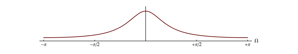
Example: Pink noise
Let the autocorrelation function of a random process be given by:
| (5.34) |
$${\varphi _{xx}}[k] = {\left( {\frac{1}{2}} \right)^{\left| k \right|}}$$
|
The power spectrum is given by:
| (5.35) |
$$\begin{array}{*{20}{l}}
{{S_{xx}}(\Omega )}&{ = \sum\limits_{k = - \infty }^{ + \infty } {{{\left( {\frac{1}{2}} \right)}^{\left| k \right|}}{e^{ - j\Omega k}}} }\\
{\,\,\,}&{ = \sum\limits_{k = - \infty }^0 {{{\left( {\frac{1}{2}} \right)}^{ - k}}{e^{ - j\Omega k}}} + \sum\limits_{k = 0}^{ + \infty } {{{\left( {\frac{1}{2}} \right)}^k}{e^{ - j\Omega k}}} - 1}\\
{\,\,\,}&{ = \frac{3}{{5 - 4\cos \Omega }}}
\end{array}$$
|
This random process is not white as the spectrum is certainly not flat. We can use other properties we have developed to determine the average value \({m_x}\) and the mean-square \(E\left\{ {{{\left| {x[n]} \right|}^2}} \right\}.\) As \(k \to \infty\) we have from Equation 5.8 that \({\varphi _{xx}}[k] \to {\left| {{m_x}} \right|^2}.\) For this example \({m_x} = 0\) and the mean-square \(E\left\{ {{{\left| {x[n]} \right|}^2}} \right\}\) is given by \({\varphi _{xx}}[0] = 1.\)
The spectra from these two examples are illustrated in Figure 5.3.
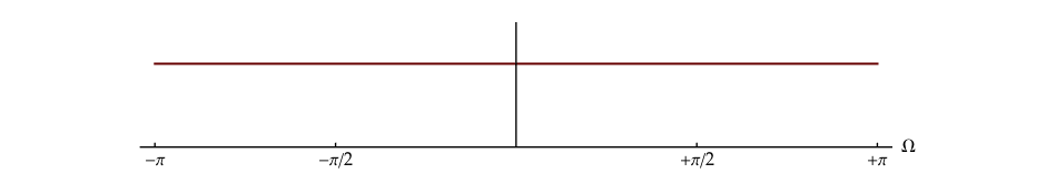
Note that we plot the spectra between \(- \pi \lt \Omega \le + \Omega\) for the simple reason that the Fourier spectrum for any discrete time signal is periodic, that is, \(X(\Omega ) = X(\Omega + 2\pi ).\) Thus it is sufficient to show or describe only one period.
Predicting the natural climate - a case study
We have developed a collection of powerful tools, in particular, the power density spectrum and the correlation function. Let us see how they can be used to gain insight into a well-known stochastic physical phenomenon, the weather.
On the cover of this iBook we show three basic concepts that have been discussed until now: a stochastic signal, its correlation function, and its power spectral density. Let us now look at some real data to see what insights these tools can give us. We again use data from the Royal Netherlands Meteorological Institute (KNMI). We use their data concerning the average daily temperature and the average daily air pressure.
We begin with the original data. For temperature, the data start at 1 January 1901 and we use the measurements until 31 December 2009. This consists of \({N_T} = 39,812\) days. For the air pressure, we use the data at the first available date which is 1 January 1902 and then (again) until 31 December 2009. This represents \({N_P} = 39,447\) days. The data are displayed in Figure 5.4.
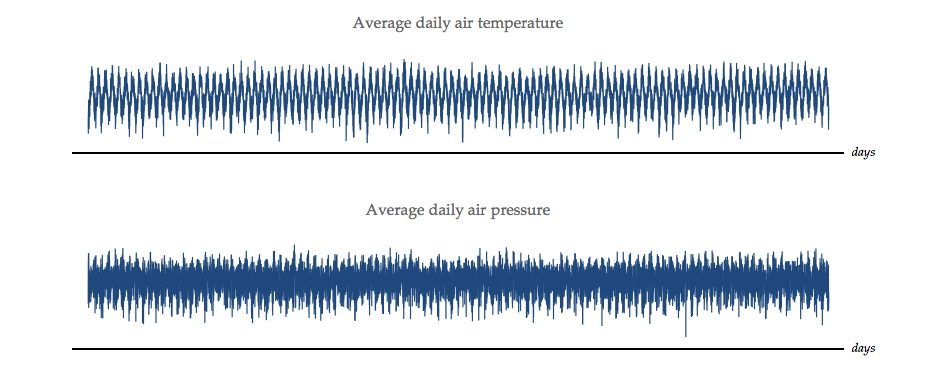
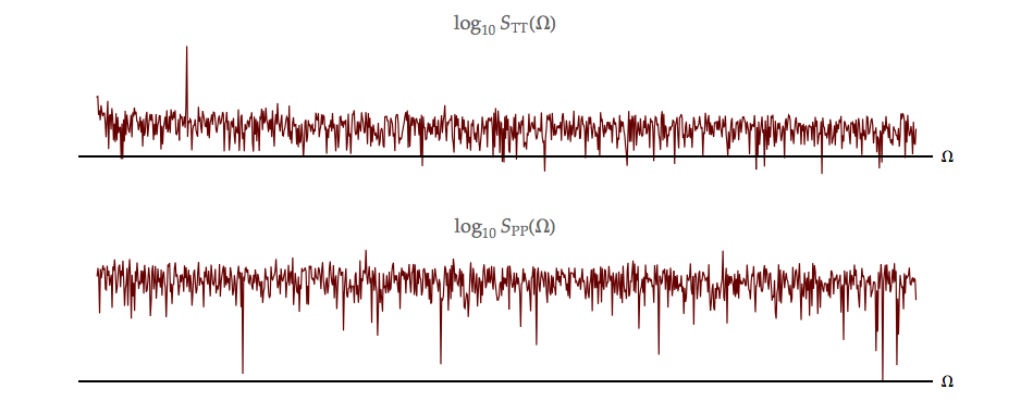
The power spectral densities, \({S_{TT}}\left( \Omega \right)\) and \({S_{PP}}\left( \Omega \right),\) for each of these stochastic signals, \(T[n]\) and \(P[n],\) can be computed using the techniques described above Equation 5.24 and in Chapter 12. They are shown in Figure 5.5. The resulting spectra reveal an interesting difference. The temperature spectrum, \({S_{TT}}\left( \Omega \right),\) shows a clear spectral peak—a significant amount of power—at frequency \({\Omega _k} = k\left( {2\pi /{N_T}} \right)\) with \(k = 109.\) This translates to a period of \({N_T}/k = 39812/109 = 365.248\) days, a familiar value. The pressure spectrum, \({S_{PP}}\left( \Omega \right),\) shows no such peak.
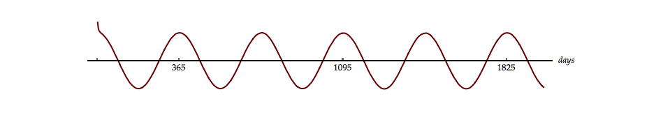
The autocorrelation functions, \({\varphi _{TT}}[k]\) and \({\varphi _{PP}}[k],\) can also be computed. See Figure 5.6. Due to the size of the data sets, we really do compute first the power spectral densities and then the autocorrelation functions as the computational efficiency of the FFT can then be exploited. (Can you estimate how much more efficient it is to use the “FFT route” to compute the autocorrelation function as opposed to a direct application of Equation 5.13?) The spectral peak identified in the power density spectrum is clearly reflected in the sinusoidal behavior of the autocorrelation function \({\varphi _{TT}}[k]\) and the one year period is obvious. A weather period of one year in daily temperatures is hardly surprising. But being able to use yearly, stochastic variations in temperature to estimate the length of the solar year with high accuracy might be surprising. The value given above, 365.248 days is only 0.002% above the currently accepted value for the solar year of 365.242 days.
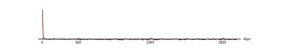
What may also be surprising is the impulse-like autocorrelation function associated with air pressure, \({\varphi _{PP}}[k].\) At the scale shown in Figure 5.6, we have essentially \({\varphi _{PP}}[k] = A\,\delta [k].\) There is virtually no month-to-month or year-to-year correlation in air pressure. If one is to be sought it should be at much shorter time scales than a one-month period.
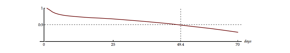
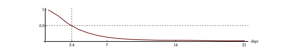
On a shorter time scale we do see short-term correlations. The average daily air temperature correlation falls to 50% of its maximum value, see Figure 5.6b, after 49.4 days. Given four seasons each of about 91 days, this is about half a season. The average daily air pressure correlation, however, falls to 50% of its maximum value after only 3.4 days, half a week. Put another way, the average daily air pressure is correlated over a significantly shorter time scale than the average daily air temperature.
We emphasize through these examples that correlation functions and spectral densities are tools and that they can be useful in understanding the structure of complex data.
Problems
Problem 5.1
Prove Equation 5.5 and the second part of Equation 5.6.
Problem 5.2
In the text we state:
- Describe a common, random process that would not have this property.
- Based upon this example, for what class of random processes would you expect that \(\mathop {\lim }\limits_{x \to \infty } \,{\gamma _{xx}}[k] \ne 0?\)
Problem 5.3
Consider the following statement:
For the ergodic random process with a mean \({m_x}\) and a variance \(\sigma _x^2,\) we have:
| (5.36) |
$$\sigma _x^2 = {\varphi _{xx}}[k = 0] - {\varphi _{xx}}[k = \infty ]$$
|
Discuss the applicability of this statement. When is it valid and when can its use lead to problems?
Problem 5.4
- Show that if \(x[n]\) is a real, ergodic process then its autocorrelation function \({\varphi _{xx}}[k]\) will be real and even.
- Show that if \({\varphi _{xx}}[k]\) is real and even then \({S_{xx}}(\Omega )\) will also be real and even.
Problem 5.5
The cross-correlation, \({\varphi _{xy}}[k],\) between two real, deterministic signals, \(x[n]\) and \(y[n],\) is given by:
- Is the cross-correlation function \({\varphi _{xy}}[k]\) even? That is, does \({\varphi _{xy}}[k] = {\varphi _{xy}}[ - k]?\) Explain your answer.
- Determine a general expression for \({S_{xy}}(\Omega ) = {\mathscr{F}}\left\{ {{\varphi _{xy}}[k]} \right\}\) in terms of \(X(\Omega )\) and \(Y(\Omega ).\)
- Determine and sketch \({\varphi _{xy}}[k]\) if \(x[n] = {a^n}u[n]\) where \(\left| a \right| < 1\) and \(y[n] = u[n - 2].\)
Problem 5.6
The following statement was found in an old textbook:
Under what circumstances are these two relations correct? Explain your reasoning.
Laboratory Exercises
Laboratory Exercise 5.1
|
We review your understanding of the difference between convolution and correlation. To start the exercise, click on the icon to the left. |
-
Oppenheim, A. V., A. S. Willsky and S. H. Nawab (1996). Signals and Systems. Upper Saddle River, New Jersey, Prentice-Hall ↩↩↩↩
-
Papoulis, A. (1965). Probability, Random Variables, and Stochastic Processes. New York, McGraw-Hill, p. 327 ↩
-
Oppenheim, A. V., R. W. Schafer and J. R. Buck (1999). Discrete-Time Signal Processing. Upper Saddle River, New Jersey, Prentice-Hall, Section 2.9 ↩
-
Actually there are some semantic issues here because white usually refers to color. If an object has a flat spectrum over the wavelength range 400 nm ≤ \(\lambda\) ≤ 750 nm, we refer to its color as white as perceived by the average observer. Frequency and wavelength are related, however, by \(f = c/\lambda.\) If the spectrum described in wavelength is flat then the frequency spectrum is not flat. The use of the term “white noise” is thus one of convention (or convenience) as opposed to color ↩
-
Porat, B. (1994). Digital Processing of Random Signals: Theory & Methods. Englewood Cliffs, New Jersey, Prentice-Hall, Section 2.5 ↩
-
Oppenheim, A. V., R. W. Schafer and J. R. Buck (1999). Discrete-Time Signal Processing. Upper Saddle River, New Jersey, Prentice-Hall, Section 2.10 ↩