Characterizing Signal-to-Noise Ratios
We now know how to characterize stochastic signals and how to determine how that characterization changes as a stochastic signal is passed through an LTI system, a linear filter. We start with an example.
Example: Filtering noise
Let the input to an LTI system be given by an ergodic process \(x[n]\) with power spectrum \({S_{xx}}(\Omega ).\) Then \({S_{yy}}(\Omega ) = {\left| {H( - \Omega )} \right|^2}{S_{xx}}(\Omega ).\) If \({\varphi _{xx}}[k] = {N_o}\delta [k]\) (white noise input) and \(h[n] = {\alpha ^n}u[n]\) with \(\alpha\) real and \(\left| \alpha \right| < 1\) then:
| (8.1) |
$$\begin{array}{l}
H(\Omega ) = \frac{1}{{1 - \alpha {e^{ - j\Omega }}}}\,\,\,\,\,\,\,\,\,\,\,{S_{xx}}(\Omega ) = {N_0}\,\,\\
{S_{yy}}(\Omega ) = {N_0}{\left| {\frac{1}{{1 - \alpha {e^{ - j\Omega }}}}} \right|^2} = \frac{{{N_0}}}{{1 + {\alpha ^2} - 2\alpha \cos \Omega }}
\end{array}$$
|
The output random process \(y[n]\) is a non-white, random process.
In the following sections we will look at several applications of these ideas as well as attempt to understand why the power density spectrum and the correlation functions play such an important role in stochastic signal processing. Further, we will focus our attention on those situations where the model is additive noise that is statistically independent of the signal.
We begin by defining a well-known measure of system performance, the signal-to-noise ratio (SNR). We make a distinction between two cases 1) where the signal is deterministic or 2) where the signal is stochastic. In either case, of course, the noise is considered to be stochastic.
SNR for deterministic signals in the presence of noise
For deterministic signals, signals where the signal amplitude is known for every time instant, we define the signal-to noise ratio as:
| (8.2) |
$$S\tilde N{R_d} = \frac{S}{N} = \frac{{\max \left| {y[n]} \right|}}{{{\sigma _{nn}}}}$$
|
or using the logarithmic (Bode) description:
| (8.3) |
$$SN{R_d} = 20\,{\log _{10}}\left( {\frac{{\max \left| {y[n]} \right|}}{{{\sigma _{nn}}}}} \right)$$
|
SNR for random signals in the presence of noise
For random signals (such as speech) which bear information but whose amplitudes cannot be predicted with certainty, we define the signal-to-noise ratio as:
| (8.4) |
$$S\tilde N{R_r} = \frac{S}{N} = \frac{{{\sigma _{ss}}}}{{{\sigma _{nn}}}}$$
|
| (8.5) |
$$SN{R_r} = 20\,{\log _{10}}\left( {\frac{{{\sigma _{ss}}}}{{{\sigma _{nn}}}}} \right)$$
|
In both cases \({\sigma _{nn}}\) is the standard deviation of the noise. In the case of random, information-bearing signals, \({\sigma _{ss}}\) is the standard deviation of the signal amplitudes.
From our earlier result, Equation 5.2, we know that
| (8.6) |
$$\sigma _{nn}^2 = {\gamma _{nn}}[0] = {\varphi _{nn}}[0] - {\left| {{m_n}} \right|^2}$$
|
We begin with the case where \({m_n} = 0\) giving \({\sigma _{nn}} = \sqrt {{\varphi _{nn}}[0]}.\) Noise with zero mean leads to a formulation for the standard deviation of the noise in terms of the autocorrelation function of the noise evaluated at \(k = 0.\) To simplify matters with respect to the case of information-bearing random signals, we will assume that their mean is also zero yielding \({\sigma _{ss}} = \sqrt {{\varphi _{ss}}[0]}.\)
The justification for this is simple. If the mean is not zero then we can express the random signal \(y[n]\) as \(y[n] = {m_y} + {y_0}[n]\) where \({m_y}\) is the (deterministic) non-zero average and \({y_0}[n]\) is a stochastic signal with the same statistics as \(y[n]\) except that its average is zero. For our discussion of SNR, we, therefore, focus on the zero-mean stochastic term.
We can now rewrite our definition using our zero-mean assumption as:
| (8.7) |
$$SN{R_d} = 10\,{\log _{10}}\left( {\frac{{\max {{\left| {y[n]} \right|}^2}}}{{{\varphi _{nn}}[0]}}} \right)$$
|
| (8.8) |
$$SN{R_r} = 10\,{\log _{10}}\left( {\frac{{{\varphi _{ss}}[0]}}{{{\varphi _{nn}}[0]}}} \right)$$
|
Example: Not too noisy
To illustrate the concept for a deterministic signal, say that a video signal generated by a known test pattern is confined to the interval 0 to 1 volt and that the noise, \(N[n],\) contaminating the video signal is 10 mv RMS. RMS means “root-mean-square” or \(\sqrt {E\left\{ {{{\left| {N[n]} \right|}^2}} \right\}}.\) From our zero mean assumption, 10 mv RMS is equivalent to \({\sigma _{nn}} = 10\) mv. According to our definition:
| (8.9) |
$$\begin{array}{*{20}{l}}
{SN{R_d}}&{ = 10\,{{\log }_{10}}\left( {\frac{{{{\left( {1\,{\rm{V}}} \right)}^2}}}{{{{\left( {{{10}^{ - 2}}\;{\rm{V}}} \right)}^2}}}} \right)}\\
{\,\,\,}&{ = 10\,{{\log }_{10}}\left( {{{10}^4}} \right) = 40\;{\rm{dB}}}
\end{array}$$
|
Example: Cocktail party noise?
We can also illustrate the concept for a random signal as follows. Let the discrete-time output of a microphone be described by \(r[n] = s[n] + N[n]\) where \(s[n]\) is a sampled, real speech signal and \(N[n]\) is sampled, real random noise from the electronics. This is shown in Figure 8.1.
The random speech signal \(s[n]\) has power density spectrum \({S_{ss}}(\Omega )\) given by:
| (8.10) |
$${S_{ss}}(\Omega ) = \frac{{{S_0}}}{{1 + {\alpha ^2} - 2\alpha \cos \Omega }}$$
|
and the independent, additive noise \(N[n]\) is characterized by:
| (8.11) |
$${S_{nn}}(\Omega ) = \frac{{{N_0}}}{{1 + {\beta ^2} - 2\beta \cos \Omega }}$$
|
The SÑRr will then follow from:
| (8.12) |
$$\begin{array}{*{20}{l}}
{{\varphi _{ss}}[0]}&{ = \frac{1}{{2\pi }}\int\limits_{ - \pi }^{ + \pi } {{S_{ss}}(\Omega )} d\Omega }\\
{\,\,\,}&{ = \frac{1}{{2\pi }}\int\limits_{ - \pi }^{ + \pi } {\frac{{{S_0}}}{{1 + {\alpha ^2} - 2\alpha \cos \Omega }}} d\Omega }\\
{\,\,\,}&{ = \frac{{{S_0}}}{{1 - {\alpha ^2}}}}
\end{array}$$
|
| (8.13) |
$$\begin{array}{*{20}{l}}
{{\varphi _{nn}}[0]}&{ = \frac{1}{{2\pi }}\int\limits_{ - \pi }^{ + \pi } {\frac{{{N_0}}}{{1 + {\beta ^2} - 2\beta \cos \Omega }}} d\Omega }\\
{\,\,\,}&{ = \frac{{{N_0}}}{{1 - {\beta ^2}}}}
\end{array}$$
|
The proof of Equation 8.12 can be found in Problem 8.1. Using Equation 8.8:
| (8.14) |
$$\begin{array}{*{20}{l}}
{SN{R_r}}&{ = 10\,{{\log }_{10}}\left( {\frac{{{S_o}/\left( {1 - {\alpha ^2}} \right)}}{{{N_o}/\left( {1 - {\beta ^2}} \right)}}} \right)}\\
{\,\,\,}&{ = 10\,{{\log }_{10}}\left( {\frac{{{S_0}}}{{{N_0}}}\,\left( {\frac{{1 - {\beta ^2}}}{{1 - {\alpha ^2}}}} \right)} \right)}
\end{array}$$
|
The two power density spectra are illustrated in Figure 8.2.
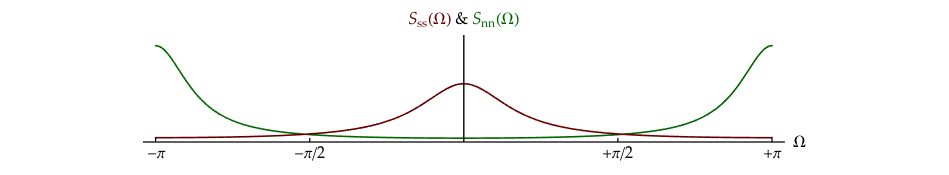
For \({S_0} = 1,\) \({N_0} = 1,\) \(\alpha = 4/7,\) and \(\beta = - 2/3,\) the SNRr = –0.84 dB.
SNR for signals and systems with Poisson noise
One very important class of noise is Poisson noise. In this case, the noise is not Gaussian, not additive, not independent of the signal, and has a mean value that is greater than zero. We would be tempted to ignore it as a mathematical oddity were it not a type of noise that is encountered in a variety of physical systems.
A Poisson process is one that describes the probability of \(n\) independent discrete events occurring in a fixed amount of time \(T\) if the time between occurrences of successive events is described by an exponential-type probability density function with a rate-parameter \(\lambda.\) The units of \(\lambda\) are events/(unit time). The value of \(T\)—the length of the observation window or the integration time—is frequently known. An exceptionally lucid derivation of the Poisson distribution can be found in Section 18.13 of Thomas1.
The emission of fluorescence photons in a labeled biological specimen, the production of photoelectrons in a CCD camera due to thermal vibrations (dark noise or dark current), and the radioactive decay of a population of identical atoms are examples of random processes governed by a Poisson distribution.
The probability of \(n\) events in \(T\) units of time is given by:
| (8.15) |
$$p(n|\lambda T) = \frac{{{{\left( {\lambda T} \right)}^n}{e^{ - \lambda T}}}}{{n!}}$$
|
For Poisson processes the signal is intrinsically noisy and needs no “help” from external sources. We define the signal-to-noise ratio as:
| (8.16) |
$$\begin{array}{*{20}{l}}
{S\tilde N{R_P} = \frac{S}{N} = \frac{\mu }{\sigma }}\\
{SN{R_P} = 20\,{{\log }_{10}}\left( {\frac{\mu }{\sigma }} \right)}
\end{array}$$
|
where \(\mu\) is the expected value of the stochastic signal and \(\sigma\) is its standard deviation. This process—whether one is talking about \(\lambda\) or \(\lambda T\)—is a one-parameter process. This means that both \(\mu\) and \(\sigma\) will be defined by \(\lambda\) (or \(\lambda T\)).
From Problem 3.4c we know that \(\mu = \lambda T\) and \(\sigma = \sqrt {\lambda T}.\) This means that:
| (8.17) |
$$\begin{array}{*{20}{l}}
{S\tilde N{R_P} = \frac{{\lambda T}}{{\sqrt {\lambda T} }} = \sqrt {\lambda T} }\\
{SN{R_P} = 20{{\log }_{10}}\left( {\sqrt {\lambda T} } \right) = 10\,{{\log }_{10}}\left( {\lambda T} \right)}
\end{array}$$
|
If we wish to increase the signal-to-noise ratio, we either have to increase the rate parameter \(\lambda\) and/or use a longer observation window \(T.\) Either approach simply means that we need more data.
The implications of these results warrant some discussion. As the strength of a Poisson signal increases—for example by using a source that emits a greater number of photons per second—so does the strength of the fluctuations. The former is measured by \(\mu\) and the latter by \(\sigma.\) This is illustrated in Figure 8.3.
In the left-hand panel you should observe that the noise increases even as the average intensity increases. The basis for this observation will be discussed in Problem 8.2. In the right-hand panel we see the fluctuations increase as the average increases. The calculation in Equation 8.17 shows, however, that as the source strength increases (from left to right) the SNR increases as well.
There is much more that can be said about Poisson noise; we will address the issue of the estimation of \(\lambda\) (or \(\lambda T\)) in an example in Chapter 11.
Problems
Problem 8.1
The autocorrelation function of a random process is given by:
| (8.18) |
$${\varphi _{xx}}[k] = {a^{\left| k \right|}}\,\,\,\,\,\,\,\,\,\,\left| a \right| < 1$$
|
- Determine the power spectral density \({S_{xx}}(\Omega ).\)
- Using \({S_{xx}}(\Omega )\) and Fourier properties prove Equation 8.12.
- What is \({m_x}\) for this process?
Problem 8.2
It has been recognized for over 150 years that the perception \(p\) of a physical stimulus \(S\) is described in many cases by:
| (8.19) |
$$\Delta p = k\frac{{\Delta S}}{S}$$
|
where \(\Delta p\) is the change in perception, \(k\) is a proportionality constant, and \(\Delta S\) represents a change in the stimulus. This is know as the Weber-Fechner Law.
- As we proceed to smaller increments in the stimulus, that is as \(\Delta S \to 0,\) what is the functional relation between \(p\) and \(S,\) that is, what is \(p(S)?\)
- For the stimulus shown in Figure 8.3, how does our observation of the noise relate to SNRp?
More information about the application of the Weber-Fechner Law to visual perception can be found in Hecht2.
Problem 8.3
The light, that passes through a test tube containing a suspension of particles in liquid, is measured by a photomultiplier and converted to a discrete-time (digital) signal. The output signal \(s[n]\) from the photomultiplier shows a stochastic variation due to the sum of two statistically independent sources: 1) the Brownian motion \(B[n]\) of the particles in the liquid, and, 2) the noise from the photomultiplier \(N[n].\) Thus:
| (8.20) |
$$s[n] = B[n] + N[n]$$
|
The autocorrelation function of the Brownian motion, that is the velocity, is modeled by:
| (8.21) |
$${\varphi _{BB}}[k] = {e^{ - \left| k \right|/D}} = {\left( {{e^{ - 1/D}}} \right)^{\left| k \right|}} = {\varepsilon ^{\left| k \right|}}$$
|
with \(0 < \varepsilon < 1.\) The autocorrelation function of the photomultiplier noise is modeled by:
| (8.22) |
$${\varphi _{NN}}[k] = \delta [k]$$
|
- What is the autocorrelation function of the signal \(s[n]\) from the photomultiplier, that is, \({\varphi _{ss}}[k]?\)
- What is the power spectral density \({S_{ss}}(\Omega )\) of the measured signal? Sketch \({S_{ss}}(\Omega ).\)
We wish to estimate \(D,\) a parameter related to the diffusion of the particles in the liquid. Our estimate of \(D\) will, of course, be sensitive to the signal-to-noise ratio SÑRr as defined in Equation 8.4.
To improve the signal-to-noise ratio we first filter the signal \(s[n]\) as shown below:
where \(h[n]\) is an ideal low-pass filter whose Fourier transform is specified in the baseband \(- \pi \lt \Omega \le + \pi\) as:
| (8.23) |
$$H(\Omega ) = {\mathscr{F}}\left\{ {h[n]} \right\} = \left\{ {\begin{array}{*{20}{c}}
1&{\left| \Omega \right| \le \pi /2}\\
0&{\left| \Omega \right| > \pi /2}
\end{array}} \right.$$
|