The Langevin Equation – A Case Study
In 1908 Prof. Paul Langevin described how a physical system modeled by a differential equation responds to a stochastic input. His work resulted in the concept of the Langevin equation. A particle of mass \(m\) is subject to random collision forces, \(f(t),\) from many small, molecules. The term \(f(t)\) is frequently described as the driving force. Further, the assumption is usually made that \(f(t)\) results from a stationary random process with a Gaussian probability density function and an autocorrelation function of the form \({\varphi _{ff}}(\tau) = {F_o}\delta (\tau ).\) Non-coincident time samples are uncorrelated. The mathematical description of \(f(t)\) is a Gaussian, white-noise, ergodic process.
The motion of the particle is held back (retarded) by a viscous, frictional force that is proportional to the velocity of the particle. The equation of motion can be written for the velocity as a function of time or the position as a function of time:
| (7.1) |
$$\begin{array}{l}
m\frac{{dv(t)}}{{dt}} = f(t) - \lambda v\\
m\frac{{{d^2}x(t)}}{{d{t^2}}} = f(t) - \lambda \frac{{dx(t)}}{{dt}}
\end{array}$$
|
where \(\lambda\) is the viscous, damping coefficient and both \(m\) and \(\lambda\) are greater than zero. This stochastic differential equation describes Brownian motion. We shall begin with the velocity, \(v(t),\) and consider only one spatial dimension.
In this case-study our intention is to illustrate how the tools we have developed can be used to analyze this random process. (See also TPM.) The tools, however, have been developed in the context of discrete-time so the first step is to transform this first-order differential equation into a difference equation. As so many problems are studied, simulated, measured, and controlled with digital systems, this is not an unreasonable first step.
From t to n
There are several procedures to transform a continuous-time LTI system—one that is based upon a linear differential equation with constant coefficients with input \(f(t)\) and output \(v(t)\) or \(x(t)\)—into a discrete-time difference equation with input \(f[n]\) and output \(v[n]\) or \(x[n].\) These include 1) impulse-invariant sampling, 2) backward-difference equation, and 3) bilinear transformation. For a thorough discussion of this topic see Section 10.8 of Oppenheim1.
Which one of the three techniques should we use? All three have advantages and disadvantages. For the purpose of this textbook, we will use the impulse-invariant sampling as it is easy to understand and leads to expressions that are easy to analyze in a case-study such as this.
Impulse-invariant sampling
If the impulse response is bandlimited, we sample the impulse response at an appropriate rate (above the Nyquist frequency) and then use z-transform techniques to produce the difference equation. Thus, if \(h(t)\) is the bandlimited impulse response of a Langevin equation whose samples are \(h[n] = h\left( {n{T_s}} \right),\) the transfer function will be given by:
| (7.2) |
$$H(z) = \sum\limits_{n = - \infty }^{ + \infty } {h[n]{z^{ - n}} = } \sum\limits_{n = - \infty }^{ + \infty } {h(n{T_s}){z^{ - n}}}$$
|
where \({T_s}\) is the suitably-chosen sampling period. The associated sampling frequency is, thereby, \({\omega _s} = 2\pi /{T_s}.\)
The impulse response of the differential equation for velocity in Equation 7.1 is causal, stable, straightforward to determine, and given by:
| (7.3) |
$${h_v}(t) = \left( {\frac{1}{m}} \right){e^{ - \left( {\lambda t/m} \right)}}u(t) = \left( {\frac{1}{m}} \right){e^{ - \left( {t/\theta } \right)}}u(t)$$
|
We have introduced the time constant \(\theta = m/\lambda\) and will use it extensively. The sampled impulse response and its z-transform are given by:
| (7.4) |
$$\begin{array}{l}
{h_v}[n] = \left( {\frac{1}{m}} \right){e^{ - \left( {\lambda {T_s}/m} \right)n}}u[n]\\
{H_v}(z) = \frac{{V(z)}}{{F(z)}} = \sum\limits_{n = - \infty }^{ + \infty } {\left( {\frac{1}{m}} \right){e^{ - \left( {\lambda {T_s}/m} \right)n}}u[n]\,{z^{ - n}}} \\
{H_v}(z) = \left( {\frac{1}{m}} \right)\sum\limits_{n = 0}^{ + \infty } {{{\left( {{e^{ - \left( {\lambda {T_s}/m} \right)}}{z^{ - 1}}} \right)}^n}} = \frac{{1/m}}{{1 - {e^{ - \left( {\lambda {T_s}/m} \right)}}{z^{ - 1}}}}
\end{array}$$
|
with a region-of-convergence (ROC) given by \(\left| z \right| > {e^{ - \lambda {T_s}/m}}.\) This leads to the difference equation:
| (7.5) |
$$v[n] - \left( {{e^{ - \left( {\lambda {T_s}/m} \right)}}} \right)v[n - 1] = \left( {\frac{1}{m}} \right)f[n]$$
|
This is the discrete-time version of the Langevin equation, Equation 7.1. The input \(f[n]\) is the Gaussian, white-noise process. See Problem 7.1 to explore an important issue related to Equation 7.5.
This all seems quite straightforward but we have neglected one significant detail. The impulse response must be bandlimited so that a finite \({T_s}\) can be chosen. But given a finite number of terms in the sum, no impulse response that is of the form \(\sum\nolimits_k {{A_k}{e^{ - {s_k}t}}u(t)}\) can be bandlimited. See Problem 7.2.
Unless the aliasing induced by the use of a finite sampling interval is negligible, the impulse invariant technique can lead to erroneous results and conclusions. This, in turn, implies that if we insist on using this technique we must sample at a very high rate. As we shall soon see, in the case of Equation 7.3, a sampling frequency of \({\omega _s} \ge 200\left( {\lambda /m} \right) = 200/\theta\) is warranted.
How big is big? How small is small?
The Langevin equation is a description appropriate for a small particle that is being battered by even smaller particles. See Section 15.5 of Reif2 for an elegant presentation of this model. To appreciate what this means let us examine the case of a gold sphere whose radius is 10 \(\mu\)m in a water bath (test tube) at a temperature of \(\Psi\) = 21 ºC. The radius of a water molecule is about 0.14 nm, about \({10^{ - 5}}\) that of the gold particle.
After a period of time the gold particle will sink to the bottom of the test tube under the force of gravity. The terminal velocity of the gold particle is, however, only 4 mm/s so we will have a few seconds to perform our measurements. In that time we will focus on lateral motion (\(x\)-direction) as opposed to axial (\(z\)-direction) motion. In the time constant \(\theta = m/\lambda\) defined in Equation 7.3, \(\lambda\) is the damping factor and according to Stokes’ Law given by:
| (7.6) |
$$\lambda = 6\pi \eta R$$
|
The parameter \(\eta\) is the dynamic viscosity of the fluid (water) and \(R\) is the “hydrodynamic” radius of the particle (gold). Substituting the appropriate values (\(\eta = 1.002\) cP, \(R = 10\) \(\mu\)m, \(m = 81\) ng) gives \(\lambda = 188.9\) \(\mu\)g/s and \(\theta\) = 428 \(\mu\)s. This is a long time compared to the average time interval between collisions of the gold sphere and water molecules which, to a rough approximation, is 10 fs. We can, therefore, consider the gold particle as being driven by a stochastic force with about \({10^{10}}\) collisions in one time constant \(\theta.\) These collisions with the gold sphere occur from all possible directions (4\(\pi\) steradians) and the large number means that the Central Limit Theorem applies and the driving force \(f(t),\) the sum of all the independent collision forces, can be modeled as having a Gaussian amplitude distribution.
Choosing the sampling period
Based upon a value for \(\theta\) that we can calculate, we now look at the appropriate value of the sampling interval \({T_s}\) for this example.
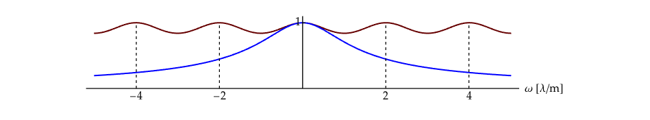
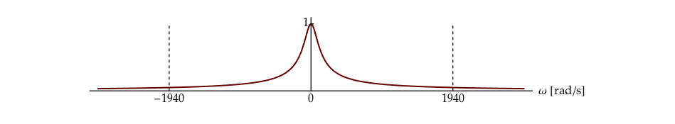
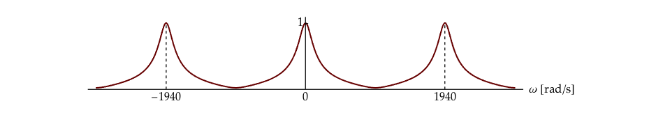
The impulse response is not bandlimited so any sampling represents undersampling. As we shall see in Figure 7.1, however, a finite choice for the sampling interval \({T_s}\) can be justified and in practice will appear to be oversampling. The “Langevin filter” associated with Equation 7.3 has a lowpass characteristic:
| (7.7) |
$$\begin{array}{l}
{h_v}(t) = \left( {\frac{1}{m}} \right){e^{ - \left( {\lambda t/m} \right)}}u(t)\\
\left| {{H_v}(\omega )} \right| = \left( {\frac{1}{m}} \right)\frac{1}{{\sqrt {{\omega ^2} + {{\left( {\lambda /m} \right)}^2}} }}
\end{array}$$
|
The frequency \({\omega _c}\) at which the amplitude-squared is down by a factor of two from its value at \(\omega = 0\) is given by \({\omega _c} = \lambda /m\) and might seem to qualify as a “highest” frequency. Using the Nyquist criterion and choosing \({\omega _s} = 2{\omega _c} = 2\lambda /m,\) however, is not enough to avoid aliasing. To do so we must choose a higher frequency \({\omega _{\max }}\) in the spectrum than \({\omega _c}.\)
If we require that the filter amplitude-squared is down by a factor of 100 (not 2) from the filter value at \(\omega = 0,\) then \({\omega _{\max }} \simeq 10{\omega _c}.\) The (Nyquist) sampling frequency is then approximated by \({\omega _s} = 2{\omega _{\max }} =\)\(2 \bullet 10{\omega _c} = 20\lambda /m.\) This sampling issue is illustrated in Figure 7.1[a,b].
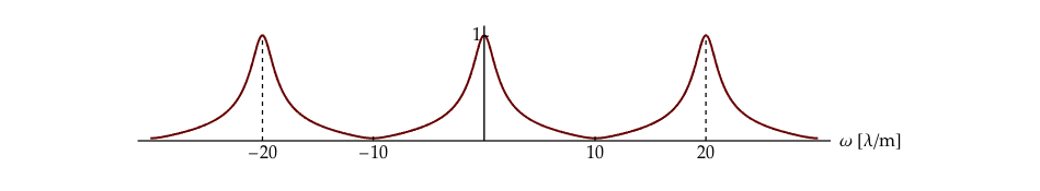
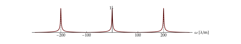
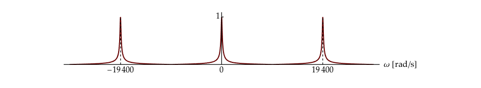
It should be clear that using a sampling frequency of \(2\lambda /m\) or \(20\lambda /m\) is insufficient to minimize aliasing. At \({\omega _s} = 200{\omega _c} = 200\lambda /m,\) as illustrated in Figure 7.1c, the aliasing is perhaps acceptable. This is the value that we shall use in the remainder of this case-study. The sampling interval is, therefore, chosen as \({T_s} = 2\pi /{\omega _s} = \pi m/100\lambda\) = 13.4 \(\mu\)s.
The question of “what is acceptable” is a tricky one. Formally, there is no “highest frequency” and thus no Nyquist frequency. Practically, a sampling frequency as illustrated in Figure 7.1c means that the damage (distortion) caused by aliasing is confined to the highest frequencies where the signal energy is already quite small. If this energy is small compared to the noise levels at these same frequencies, then the choice of \({T_s}\) can be considered “acceptable”. This is not a mathematical choice, however, but an engineering one. The comparison of signal energy and noise energy is the subject of Chapter 8.
The Langevin velocity equation
Let us begin with the velocity equation, its original form, and our difference equation based upon the impulse-invariant transformation:
| (7.8) |
$$\begin{array}{*{20}{l}}
{m\frac{{dv(t)}}{{dt}} + \lambda v(t) = f(t)}\\
{v[n] - \left( {{e^{ - \left( {\lambda {T_s}/m} \right)}}} \right)v[n - 1] = \left( {\frac{1}{m}} \right)f[n]}
\end{array}$$
|
The driving force is Gaussian, white noise with the following characteristics:
| (7.9) |
$$\begin{array}{l}
{\varphi _{ff}}[k] = {F_o}\delta [k]\\
{S_{ff}}(\Omega ) = {F_o}
\end{array}$$
|
We now appeal to Equation 5.8, Equation 5.2, and Equation 5.4 which are summarized below:
| (7.10) |
$$\begin{array}{l}
\mathop {\lim }\limits_{k \to \infty } \left\{ {{\varphi _{ff}}[k]} \right\} = {\left| {{m_f}} \right|^2}\\
{\gamma _{ff}}[0] = {\varphi _{ff}}[0] - {\left| {{m_f}} \right|^2} = \sigma _f^2
\end{array}$$
|
Substituting the values from Equation 7.9 into Equation 7.10 yields the results that \({m_f} = \left\langle {f[n]} \right\rangle = 0\) and \({\sigma _f} = \sqrt {{F_o}}.\) The average value of the driving force is zero. In this one-dimensional system there is—on the average—just as much force coming from the left as from the right. The standard deviation of the force is \(\sqrt {{F_o}}.\) But this describes the input driving force. What are the characteristics of the random process that describes the particle velocity?
Autocorrelation function
To answer this question we need to compute the autocorrelation of the velocity \({\varphi _{vv}}[k]\) and its power spectral density \({S_{vv}}(\Omega ).\) The autocorrelation follows from Equation 6.15, specifically \({\varphi _{vv}}[k] = {\varphi _{ff}}[k] \otimes {\varphi _{hh}}[k]\) where \({\varphi _{hh}}[k]\) is the autocorrelation function of the deterministic impulse response of the Langevin filter. That impulse response follows from Equation 7.8 and is given by:
| (7.11) |
$${h_v}[n] = \left( {\frac{1}{m}} \right){e^{ - (\lambda {T_s}/m)n}}u[n] = \left( {\frac{1}{m}} \right){\rho ^n}u[n]$$
|
where we have set \(\rho = {e^{ - \left( {\lambda {T_s}/m} \right)}}\) and clearly \(0 < \rho < 1.\) It follows that:
| (7.12) |
$$\begin{array}{*{20}{l}}
{{\varphi _{hh}}[k]}&{ = {{\left( {\frac{1}{m}} \right)}^2}\sum\limits_{n = 0}^{ + \infty } {{\rho ^{2n + \left| k \right|}}} }\\
{\,\,\,}&{ = {{\left( {\frac{1}{m}} \right)}^2}\left( {\frac{1}{{1 - {\rho ^2}}}} \right){\rho ^{\left| k \right|}}}
\end{array}$$
|
At this point you should notice some similarities to calculations performed in Equation 5.18 and Equation 5.19 including the use of the evenness of the autocorrelation function.
Power spectral density
The power spectral density associated with the deterministic signal \(h[n],\) \({S_{hh}}(\Omega ) = {\mathscr{F}}\left\{ {{\varphi _{hh}}[k]} \right\},\) is given by:
| (7.13) |
$$\begin{array}{*{20}{l}}
{{S_{hh}}(\Omega )}&{ = {\mathscr{F}}\left\{ {{{\left( {\frac{1}{m}} \right)}^2}\left( {\frac{1}{{1 - {\rho ^2}}}} \right){\rho ^{\left| k \right|}}} \right\}}\\
{\,\,\,}&{ = {{\left( {\frac{1}{m}} \right)}^2}\left( {\frac{1}{{1 + {\rho ^2} - 2\rho \cos \Omega }}} \right)}
\end{array}$$
|
Note that the real and even autocorrelation function \({{\varphi _{hh}}[k]}\) has led to a real and even power spectral density \({S_{hh}}(\Omega ).\)
The next step is to calculate \({{\varphi _{vv}}[k]}\) and \({S_{vv}}(\Omega )\) but that is straightforward given Equation 6.15 and Equation 7.9.
| (7.14) |
$$\begin{array}{*{20}{l}}
{{\varphi _{vv}}[k]}&{ = {\varphi _{ff}}[k] \otimes {\varphi _{hh}}[k]}\\
{\,\,\,}&{ = {F_o}\delta [k] \otimes {\varphi _{hh}}[k] = {F_o}{\varphi _{hh}}[k]}\\
{\,\,\,}&{ = {{\left( {\frac{1}{m}} \right)}^2}\left( {\frac{{{F_o}}}{{1 - {\rho ^2}}}} \right){\rho ^{\left| k \right|}}}\\
{\,\,\,}&{\,\,\,}\\
{{S_{vv}}(\Omega )}&{ = {S_{ff}}(\Omega ){S_{hh}}(\Omega ) = {F_o}{S_{hh}}(\Omega )}\\
{\,\,\,}&{ = {{\left( {\frac{1}{m}} \right)}^2}\left( {\frac{{{F_o}}}{{1 + {\rho ^2} - 2\rho \cos \Omega }}} \right)}
\end{array}$$
|
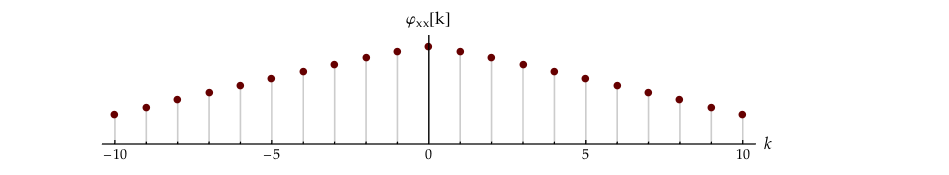
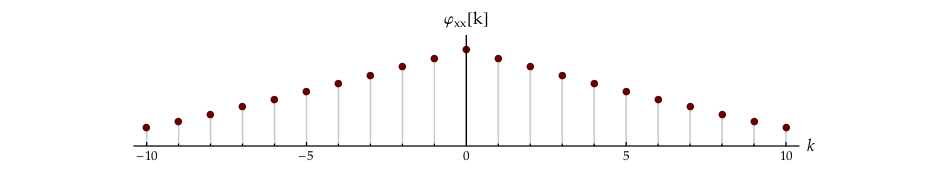
These two descriptions of the filtered random process—a white, Gaussian process filtered through the Langevin velocity equation—are illustrated in Figure 7.2.
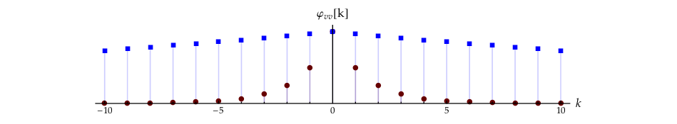
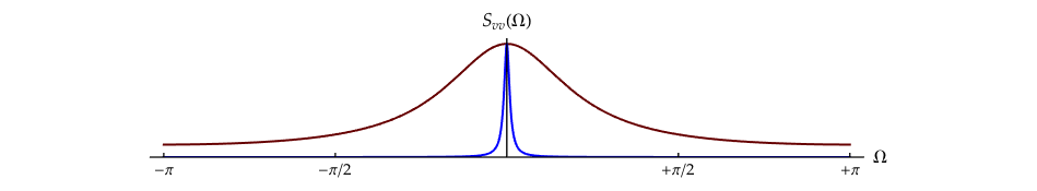
It should be clear that although the driving force is white noise, the velocity process is pink noise as described in Example: Pink Noise.
Descriptive statistics – mean and standard deviation
Having the autocorrelation function and the power spectral density, we can now calculate the mean and standard deviation of the filtered random process. There are two ways to arrive at the mean. We can use Equation 7.10 with Equation 7.12 and Equation 7.14 in which case we have:
| (7.15) |
$${\left| {{m_v}} \right|^2} = \mathop {\lim }\limits_{k \to \infty } \left\{ {{\varphi _{vv}}[k]} \right\} = 0$$
|
That is, the mean is 0. Alternatively, we can use Equation 6.9 and Equation 7.4 to give:
| (7.16) |
$$\begin{array}{*{20}{l}}
{{m_v}}&{ = {m_f}\,{H_v}(\Omega = 0) = {m_f}\,{H_v}(z = 1)}\\
{\,\,\,}&{ = 0\left( {\frac{{1/m}}{{1 - {e^{ - (\lambda {T_s}/m)}}}}} \right) = 0}
\end{array}$$
|
Either way, a mean of zero makes sense. The driving force pushes the particle left and right and the Langevin equation smooths this motion. But the smoothing does not change the average velocity.
The standard deviation comes from:
| (7.17) |
$$\begin{array}{*{20}{l}}
{\sigma _v^2}&{ = {\gamma _{vv}}[0] = {\varphi _{vv}}[0] - {{\left| {{m_v}} \right|}^2}}&{\,\,\,}\\
{\,\,\,}&{ = {\varphi _{vv}}[0] = {{\left( {\frac{1}{m}} \right)}^2}\left( {\frac{{{F_o}}}{{1 - {\rho ^2}}}} \right)}& \Rightarrow \\
{{\sigma _v}}&{ = \frac{1}{m}\sqrt {\frac{{{F_o}}}{{1 - {e^{ - 2\lambda {T_s}/m}}}}} }&{\,\,\,}
\end{array}$$
|
The standard deviation changes, something we should expect from the filtering associated with the Langevin equation and our experience with Laboratory Exercise 6.1 in Chapter 6.
It is instructive to compare this discrete-time result to the continuous time result. We offer—without proof—that the various equations to describe the filtering of random processes and the calculation of various statistical descriptions are the same in continuous time as in discrete time. You are, of course, welcome to derive these results using the same methods we have used in the previous chapters. See Problem 7.3.
Starting from Equation 7.1 and Equation 7.3 we have the results summarized in Table 1.
| Description | Continuous-time | Discrete-time |
|---|---|---|
| ${h_v}$ | $\frac{1}{m}{e^{ - \lambda t/m}}u(t)$ | $\frac{1}{m}{\rho ^n}u[n]$ |
| ${H_v}$ | $\frac{1}{{ms + \lambda }}$ | $\frac{1}{m}\left( {\frac{1}{{1 - \rho {z^{ - 1}}}}} \right)$ |
| ${\varphi _{hh}}$ | $\left( {\frac{1}{{2m\lambda }}} \right){e^{ - \lambda \lvert \tau \rvert/m}}$ | ${\left( {\frac{1}{m}} \right)^2}\left( {\frac{1}{{1 - {\rho ^2}}}} \right){\rho ^{\lvert k \rvert}}$ |
| ${\varphi _{vv}}$ | ${F_o}{\varphi _{hh}}(\tau )$ | ${F_o}{\varphi _{hh}}[k]$ |
| ${S_{vv}}$ | ${\left( {\frac{1}{m}} \right)^2}\frac{{{F_o}}}{{{\omega ^2} + {{\left( {\lambda /m} \right)}^2}}}$ | ${\left( {\frac{1}{m}} \right)^2}\left( {\frac{{{F_o}}}{{1 + {\rho ^2} - 2\rho \cos \Omega }}} \right)$ |
| ${\lvert {{m_v}} \rvert^2} = \mathop {\lim }\limits_{\tau ,\,k \to \infty } \left\{ {{\varphi _{vv}}} \right\}$ | 0 | 0 |
| $\begin{aligned}\sigma_v^2 &= \left( \varphi_{vv} - \lvert m_v \rvert^2 \right) \rvert_{\tau ,k = 0}\\ &= \langle v^2 \rangle \end{aligned}$ | $\frac{{{F_o}}}{{2m\lambda }}$ | ${\left( {\frac{1}{m}} \right)^2}\left( {\frac{{{F_o}}}{{1 - {\rho ^2}}}} \right)$ |
The result for the average value of the velocity is the same; the mean value of the velocity is zero. The result for the continuous-time standard deviation (or variance \(\sigma _{v,a}^2\)) differs from the discrete-time standard deviation (or variance \(\sigma _{v,d}^2\)) where “\(a\)” stands for analog (continuous-time) and “\(d\)” for digital (discrete-time).
| (7.18) |
$$\begin{array}{*{20}{l}}
{\sigma _{v,a}^2}&{ = \frac{{{F_o}}}{{2m\lambda }}}\\
{\sigma _{v,d}^2}&{ = \frac{1}{{{m^2}}}\left( {\frac{{{F_o}}}{{1 - {\rho ^2}}}} \right) = \frac{1}{{{m^2}}}\left( {\frac{{{F_o}}}{{1 - {e^{ - 2\lambda {T_s}/m}}}}} \right)}
\end{array}$$
|
We pay a price for using discrete-time techniques, the perhaps unexpected term \(1 - {\rho ^2}\) in the denominator of Equation 7.18. This term can, however, asymptotically resemble the term in Table 7.1.
As the sampling rate increases, as \({T_s} \to 0,\) we have:
| (7.19) |
$$\begin{array}{*{20}{l}}
{\mathop {\lim }\limits_{{T_s} \to 0} \left\{ {\sigma _{v,d}^2} \right\}}&{ = \mathop {\lim }\limits_{{T_s} \to 0} \left\{ {\frac{1}{{{m^2}}}\left( {\frac{{{F_o}}}{{1 - {e^{ - 2\lambda {T_s}/m}}}}} \right)} \right\}}\\
{\,\,\,}&{ \approx \frac{{{F_o}}}{{{m^2}}}\left( {\frac{1}{{1 - (1 - 2\lambda {T_s}/m)}}} \right)}\\
{\,\,\,}&{ \approx \frac{{{F_o}}}{{2m\lambda {T_s}}} = \frac{1}{{{T_s}}}\sigma _{v,a}^2}
\end{array}$$
|
Note that we have used the Taylor series linearization of \({\rho ^2}\) as \({T_s} \to 0.\) This suggests using a sampling interval such that \({T_s} < < m/2\lambda = \theta /2.\) We have met this condition with our earlier choice of \({T_s} = 2\pi /{\omega _s} = \pi m/100\lambda.\) We can then calculate the variance of the physical (analog) velocity process from our (digital) data, \(\sigma _{v,a}^2 = {T_s}\,\sigma _{v,d}^2.\)
Before proceeding with the Langevin position equation, one more observation is in order. The variance of the continuous-time velocity is the mean-square velocity of the particle with mass \(m\) in the water bath at temperature \(\Psi.\) The battering of the particle by water molecules is caused by the thermal motion of the molecules. Even though the particle is in thermal equilibrium with its surroundings, the battering continues. From the Equipartition Theorem of thermal physics we know that each degree-of-freedom of motion has as an average kinetic energy of \({k_B}\Psi /2\) due to thermal effects—see Feynman3—where \({k_B} = 1.380658 \times {10^{ - 23}}\) J/K is the Boltzmann constant. With \(K{E_x}\) denoting the average kinetic energy of translational motion in the \(x\) direction, this means:
| (7.20) |
$$\begin{array}{*{20}{l}}
{\frac{{{F_o}}}{{2m\lambda }}}&{ = \sigma _{v,a}^2 = \left\langle {v_x^2} \right\rangle = \frac{{2\,K{E_x}}}{m} = \frac{{{k_B}\Psi }}{m}\,\,\,\, \Rightarrow }\\
{{F_o}}&{ = 2\lambda {k_B}\Psi }
\end{array}$$
|
The second line in Equation 7.20 is important. Based upon the dynamic viscosity, the equilibrium temperature, and the Boltzmann constant, we can assign a specific physical value to \({{F_o}},\) a term that has, until now, been a simple scale factor.
The Langevin position equation
At first glance one might expect that analyzing the Langevin position equation might simply be “more of the same”. As we shall see, however, this equation offers some important insights into phenomena such as Brownian motion.
We start with the causal, stable position equation in continuous time:
| (7.21) |
$$\begin{array}{l}
m\frac{{{d^2}x(t)}}{{d{t^2}}} = f(t) - \lambda \frac{{dx(t)}}{{dt}}\\
{H_x}(s) = \frac{1}{{m{s^2} + \lambda s}}
\end{array}$$
|
The impulse response \({h_x}(t)\) follows from:
| (7.22) |
$$\begin{array}{l}
{H_x}(s) = \frac{1}{{m{s^2} + \lambda s}} = \frac{1}{\lambda }\left( {\frac{1}{s} - \frac{1}{{s + \lambda /m}}} \right)\,\,\,\,\, \Rightarrow \\
{h_x}(t) = \frac{1}{\lambda }u(t) - \frac{1}{\lambda }{e^{ - \lambda t/m}}u(t)
\end{array}$$
|
Using the impulse-invariant technique yields:
| (7.23) |
$$\begin{array}{*{20}{l}}
{{h_x}[n]}&{ = \frac{1}{\lambda }u[n] - \frac{1}{\lambda }{{\left( {{e^{ - \lambda {T_s}/m}}} \right)}^n}u[n]}&{}\\
{\,\,\,}&{ = \frac{1}{\lambda }u[n] - \frac{1}{\lambda }{\rho ^n}u[n]}& \Rightarrow \\
{{H_x}(z)}&{ = \frac{{1{\rm{/}}\lambda }}{{1 - {z^{ - 1}}}} - \frac{{1{\rm{/}}\lambda }}{{1 - \rho {z^{ - 1}}}}}&{}\\
{\,\,\,}&{ = \frac{1}{\lambda }\left( {\frac{{{z^{ - 1}}(1 - \rho )}}{{1 - {z^{ - 1}}(1 + \rho ) + \rho {z^{ - 2}}}}} \right)}&{}
\end{array}$$
|
Again we have used \(\rho = {e^{ - (\lambda {T_s}/m)}}.\) The difference equation relating driving force \(f[n]\) to position \(x[n]\) is thus given by:
| (7.24) |
$$\begin{array}{l}
x[n] - (1 + \rho )x[n - 1] + \rho x[n - 2]\\
\,\,\,\,\,\,\,\, = \left( {\frac{{1 - \rho }}{\lambda }} \right)f[n - 1]
\end{array}$$
|
Expected value
The average value of the position \({m_x},\) using the property that \(\Omega = 0\) corresponds to \(z = {\left. {{e^{j\Omega }}} \right|_{\Omega = 0}} = 1,\) is straightforward to calculate:
| (7.25) |
$$\begin{array}{*{20}{l}}
{{m_x}}&{ = {m_f}\,{H_x}(\Omega = 0) = {m_f}\,{H_x}(z = 1)}\\
{\,\,\,}&{ = 0\left( {\frac{{1 - \rho }}{\lambda }} \right)\left( {\frac{1}{0}} \right) = indeterminate}
\end{array}$$
|
What is happening here? First, this is not a consequence of the transformation from continuous time to discrete time. The value of \({H_x}(\omega )\) is also indeterminate for \(\omega = 0.\) We can better understand this result if we look at the impulse response of the difference equation, Equation 7.23.
| (7.26) |
$${h_x}[n] = \left( {\frac{1}{\lambda }} \right)u[n] - \left( {\frac{1}{\lambda }} \right){\rho ^n}u[n]$$
|
The form of this impulse response brings us back to the discussion in Chapter 5. The first term is dependent on \(u[n]\) whose Fourier transform—as we saw in Equation 5.21—has singularities at \(\Omega = 0.\) It is these singularities that cause our problem.
Nevertheless, our intuition suggests that the mean \({m_x}\) should be zero. The random process associated with \(f[n]\) has a zero mean, \({m_f} = \left\langle {f[n]} \right\rangle = 0,\) so the positive values should be “cancelled” by the negative values. As we have assumed that \(f[n]\) has a Gaussian probability density function \(N\left( {\mu = 0,\sigma = \sqrt {{F_o}} } \right),\) we can show that this is an example of a filtered Gaussian random walk.
The first term in \({h_x}[n]\) in Equation 7.26, \({h_1}[n] = \left( {1/\lambda } \right)u[n]\) implies that the position after \(n\) steps involves the sum of that number of independent steps:
| (7.27) |
$$\begin{array}{*{20}{l}}
{{x_1}[n]}&{ = \left( {\frac{1}{\lambda }} \right)u[n] \otimes f[n] = \left( {\frac{1}{\lambda }} \right)\sum\limits_{k = - \infty }^{ + \infty } {f[k]u[n - k]} }\\
{\,\,\,}&{ = \left( {\frac{1}{\lambda }} \right)\sum\limits_{k = 0}^n {f[k]} }
\end{array}$$
|
We assume here that the particle with mass \(m\) starts at position zero at time zero, \(x[0] = 0,\) and that the random driving force starts at time zero, \(f[n] = 0\) for \(n < 0.\) The term \(\sum\nolimits_k {f[k]}\) represents the sum of \(n\) independent, identically-distributed, Gaussian random variables: a Gaussian random walk. Random walks have been studied extensively and a lucid discussion can be found in Cox4.
For a random walk where each step has an average value of zero, the expected value of the particle position after \(n\) steps is likewise zero. The second term in \({h_x}[n]\) in Equation 7.26 is easier; the output of this component of the Langevin filter has a mean of zero. This can be seen through application of Equation 6.9 with \({m_f} = 0.\)
By identifying the first term in \({h_x}[n]\) (Equation 7.26) as a Gaussian random walk problem, we have demonstrated that the mean value of the position in the Langevin position equation is zero, \({m_x} = \left\langle {x[n]} \right\rangle = 0.\)
Autocorrelation function
We are now in a position to work with the autocorrelation function. Again we refer to the methodology developed in Chapter 5 for a deterministic signal, specifically Equation 5.14, and to the impulse response of the Langevin position equation, Equation 7.26. For the deterministic signal we had:
| (7.28) |
$$x[n] = u[n] - {\left( {\frac{1}{2}} \right)^n}u[n]$$
|
and for the Langevin position equation:
| (7.29) |
$${h_x}[n] = \left( {\frac{1}{\lambda }} \right)u[n] - \left( {\frac{1}{\lambda }} \right){\rho ^n}u[n]$$
|
The similarity of the two equations should be clear. This means that, referring to Equation 5.19 and using the windowing function \(w[n]\) and Equation 7.14, we can write the autocorrelation function as:
| (7.30) |
$${\varphi _{xx}}[k] = \frac{{{F_o}}}{{{\lambda ^2}}}\left( {\mathop {\lim }\limits_{N \to \infty } N - \left| k \right| - \left( {\frac{{\rho + {\rho ^2} + {\rho ^{\left| k \right| + 1}}}}{{1 - {\rho ^2}}}} \right)} \right)$$
|
In order to show that \({\varphi _{xx}}[k]\) grows linearly with \(N\) we do not replace it by its limit.
The autocorrelation is displayed in Figure 7.3. It is important to realize that while it may look quite similar to Figure 5.2, it differs in an important way. The example that was developed in Chapter 5 was the autocorrelation function of a deterministic signal \(x[n].\) The result in Equation 7.30 is the autocorrelation function of the stochastic signal \(x[n]\) found through the Langevin equation.
We have determined the mean value of the random process \({m_x} = \left\langle {x[n]} \right\rangle = 0\) and we now have the autocorrelation function of that random process in the form of Equation 7.30.
Power spectral density
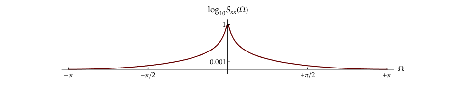
Starting from Equation 6.21 and Equation 7.29 we can compute the power spectral density \({S_{xx}}(\Omega ).\) See Problem 7.6.
| (7.31) |
$$\begin{array}{*{20}{l}}
{{S_{xx}}(\Omega )}&{ = {{\left| {{H_x}(\Omega )} \right|}^2}{S_{ff}}(\Omega )\; = {{\left| {{H_x}(\Omega )} \right|}^2}{F_o}}\\
{\,\,\,}&{ = \frac{{{F_o}{{(1 - \rho )}^2}{{\csc }^2}(\Omega /2)}}{{{{(2\lambda )}^2}(1 + {\rho ^2} - 2\rho \cos \Omega )}}}
\end{array}$$
|
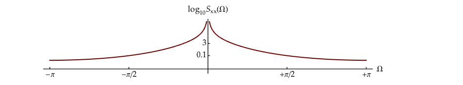
This result including its behavior at \(\Omega = 0\) is shown in Figure 7.4.
Using Equation 7.10 we can determine the variance—the mean-square dispersion \(\left\langle {{x^2}} \right\rangle\)—of the random process.
| (7.32) |
$$\begin{array}{*{20}{l}}
{\sigma _x^2}&{ = {\gamma _{xx}}[0] = {\varphi _{xx}}[0] - {{\left| {{m_x}} \right|}^2} = {\varphi _{xx}}[0] - {0^2}}\\
{\,\,\,}&{ = \frac{{{F_o}}}{{{\lambda ^2}}}\left( {\mathop {\lim }\limits_{N \to \infty } N - \left( {\frac{{2\rho + {\rho ^2}}}{{1 - {\rho ^2}}}} \right)} \right) = \left\langle {{x^2}} \right\rangle }
\end{array}$$
|
The size of the window and the number of independent steps that are added together in Equation 7.27 are the same, \(N.\) This means that for large values of \(N,\) the variance grows as \(N\) and the standard deviation grows as \(\sqrt N.\) This coincides with our knowledge of the Gaussian random walk and Brownian motion, an average displacement of zero and a standard deviation that grows as \(\sqrt N\) and is, therefore, unbounded.
To repeat what we mentioned in Chapter 5, the mathematics may indicate that we are dealing with an “ill-behaved” mathematical problem but this problem can, in fact, be a description of a real physical system and amenable to analysis and interpretation.
As we saw in Equation 7.19, examining what happens as the sampling rate increases, as \({T_s} \to 0,\) can provide additional insight into the relation between the analog world and the digital world. Using the same linearization procedure yields:
| (7.33) |
$$\sigma _x^2 = \frac{{{F_o}}}{{{\lambda ^2}}}\left( {\mathop {\lim }\limits_{N \to \infty } N - \left( {\frac{{3m}}{{2\lambda {T_s}}} - 2} \right)} \right)$$
|
In Figure 7.1, we demonstrated that a sufficiently small value of the sampling interval is given by \({T_s} = \pi m/100\lambda.\) The approximation that we are in a region where the \(\sqrt N\) behavior dominates is thus given by:
| (7.34) |
$$N > > \frac{3}{2}\left( {\frac{m}{{\lambda {T_s}}}} \right) = \frac{{150}}{\pi }$$
|
The total amount of time, \({T^*},\) that passes before we are in this region is characterized by:
| (7.35) |
$${T^*} > > \frac{3}{2}\left( {\frac{m}{{\lambda {T_s}}}} \right){T_s} = \frac{3}{2}\left( {\frac{m}{\lambda }} \right) = \frac{3}{2}\theta$$
|
For the numerical example presented earlier where \(\theta = 428\mu\)s, this implies that starting at time zero where \(x[0] = 0,\) Brownian motion with its \(\sqrt N\) behavior will dominate the digital data when \({T^*} > > 642\mu\)s.
As we saw with Table 7.1, it can be instructive to compare our discrete-time results to their continuous-time counterparts. These are summarized in Table 7.2.
| Description | Continuous-time | Discrete-time |
|---|---|---|
| ${h_x}$ | $\frac{1}{\lambda }u(t) - \frac{1}{\lambda }{e^{ - \lambda t/m}}u(t)$ | $\frac{1}{\lambda }u[n] - \frac{1}{\lambda }{\left( {{e^{ - \lambda {T_s}/m}}} \right)^n}u[n]$ |
| ${H_x}$ | $\frac{1}{{m{s^2} + \lambda s}}$ | $\frac{1}{\lambda }\left( {\frac{{{z^{ - 1}}(1 - \rho )}}{{1 - {z^{ - 1}}(1 + \rho ) + \rho {z^{ - 2}}}}} \right)$ |
| ${\varphi _{hh}}$ | $\frac{1}{{{\lambda ^2}}}(\mathop {\lim }\limits_{T \to \infty } T - \lvert \tau \rvert$
$ - \frac{m}{\lambda }(2 + {e^{ - \lambda \lvert \tau \rvert/m}}))$ |
$\frac{1}{{{\lambda ^2}}}(\mathop {\lim }\limits_{N \to \infty } N - \lvert k \rvert$
$ - (\frac{{\rho + {\rho ^2} + {\rho ^{\lvert k \rvert + 1}}}}{{1 - {\rho ^2}}}))$ |
| ${\varphi _{xx}}$ | ${F_o}{\varphi _{hh}}(\tau )$ | ${F_o}{\varphi _{hh}}[k]$ |
| ${S_{xx}}$ | $\left( {\frac{1}{{{m^2}}}} \right)\left( {\frac{1}{{{\omega ^2}}}} \right)\frac{{{F_o}}}{{{\omega ^2} + {{\left( {\lambda /m} \right)}^2}}}$ | $\frac{{{{(1 - \rho )}^2}{{\csc }^2}(\Omega /2)}}{{{{(2\lambda )}^2}(1 + {\rho ^2} - 2\rho \cos \Omega )}}$ |
| ${\lvert {{m_x}} \rvert^2} = \mathop {\lim }\limits_{\tau ,\,k \to \infty } \left\{ {{\varphi _{xx}}} \right\}$ | 0 | 0 |
| $\begin{aligned}\sigma_x^2 &= \left( \varphi_{xx} - \lvert m_x \rvert^2 \right) \rvert_{\tau ,k = 0}\\ &= \langle x^2 \rangle \end{aligned}$ | $\frac{{{F_o}}}{{{\lambda ^2}}}\left( {\mathop {\lim }\limits_{T \to \infty } T - \left( {\frac{{3m}}{\lambda }} \right)} \right)$ | $\frac{{{F_o}}}{{{\lambda ^2}}}\left( {\mathop {\lim }\limits_{N \to \infty } N - \left( {\frac{{2\rho + {\rho ^2}}}{{1 - {\rho ^2}}}} \right)} \right)$ |
To compare the variance estimates as we did in Equation 7.19, we look at the situation where \({T_s} \to 0.\)
| (7.36) |
$$\begin{array}{*{20}{l}}
{\sigma _{x,a}^2}&{ = \frac{{{F_o}}}{{{\lambda ^2}}}\left( {\mathop {\lim }\limits_{T \to \infty } T - \left( {\frac{{3m}}{\lambda }} \right)} \right)}\\
{\sigma _{x,d}^2}&{ = \frac{{{F_o}}}{{{\lambda ^2}}}\left( {\mathop {\lim }\limits_{N \to \infty } N - \left( {\frac{{3m}}{{2\lambda {T_s}}} - 2} \right)} \right)}
\end{array}$$
|
The results are similar to what we saw before. The \(\sqrt T\) or \(\sqrt N\) behavior of the standard deviation dominates after a sufficient observation time. Further, the relative behavior of the two variances can be described by \(\sigma _{x,a}^2 \propto {T_s}\sigma _{x,d}^2.\)
This is the second time that we have seen this relation between the continuous-time and the discrete-time and it will appear in the next section as well. This may surprise you as it appears that the units of the stochastic variable are not compatible. If, on the left side, the variance has the unit \({\left( {m/s} \right)^2}\) as in the velocity equation Equation 7.19, then it should have that same unit for the variance on the right side as well. And the same holds for position. If on the left side, the variance has the unit \({m^2}\) as in the position equation Equation 7.36 then it should also be \({m^2}\) for the variance on the right side. So how does the \({T_s}\) fit in? We will explore this issue in Problem 7.8.
Tethered particle motion
While the Langevin equation was described more than 100 years ago, the concepts introduced are still used in modern studies. To further our appreciation for how the processing of stochastic signals can yield insights into, for example, the biophysical properties of DNA, let us look at how a variant of the Langevin equation is used.
The motion of a gold particle in a fluid provides a mechanism to study the dynamic behavior of polymers such as double-stranded DNA (dsDNA). In dynamic studies one can see how DNA is affected by ionic concentrations (e.g. \({\rm{M}}{{\rm{g}}^{ + + }}\)) or by repair and maintenance proteins such as RecA. In the original model embodied in the Langevin equation, Equation 7.1, the particle is free to move in the fluid. If, however, the particle is attached to one end of a polymer—a macromolecule that is composed of a chain of essentially identical subunits—and the other end of the polymer is attached to a substrate, then the motion of the particle will no longer be free. This is referred to as tethered particle motion (TPM) and is illustrated in Figure 7.5. See Lindner5.
The tether constrains the particle from free motion through two mechanisms. First, the particle cannot move further away from the attachment point of the molecule than the total molecule length \(L.\) If the molecule has a length of \(L = 1660\) nm then the three-dimensional envelope of possible positions is a hemisphere of radius 1660 nm. (There is a small correction necessary because the particle cannot penetrate the substrate but we shall ignore this volume exclusion effect.)
Second, within this hemisphere small displacements of the particle in the fluid due to thermal collisions with the water molecules are restrained by a spring-like (Hookean) force, \({f_{mol}} = - kx\) exerted by the macromolecule. This leads to the modification of the Langevin model presented in Equation 7.1:
| (7.37) |
$$m\frac{{{d^2}x(t)}}{{d{t^2}}} = f(t)\,\,\,\underbrace { - \lambda \frac{{dx(t)}}{{dt}}}_{frictional\,force}\,\,\,\underbrace { - kx}_{Hookean\,force}$$
|
where \(k\) is the spring constant associated with the macromolecule. The three parameters \(\left( {m,\lambda ,k} \right)\) are all positive. Further, the first two deal with the particle and the fluid while the third one, \(k,\) is a direct property of the macromolecular tether and thus experiments with the tethered particle can reveal properties of the macromolecule.
A simulation of the three-dimensional motion involved is shown in Movie 7.1. See Lindner5.
Real data as recorded from an \(R = 40\) nm gold sphere through a darkfield microscope are shown in Movie 7.2. See Dietrich6.
It is the Langevin equation extended with a spring force that describes the motion seen in Movie 7.1 and Movie 7.2. The transfer function of the modified Langevin equation is:
| (7.38) |
$${H_x}(s) = \frac{1}{{m{s^2} + \lambda s + k}}$$
|
As in the Langevin position equation, this is a second-order linear differential equation but this time containing the spring constant. This type of second-order system is well-known. See Section 6.5.2 of Oppenheim7. There are three types of possible behavior depending upon the value of the discriminant \({\left( {\lambda /2m} \right)^2} - \left( {k/m} \right).\) These are:
| (7.39) |
$$\begin{array}{*{20}{l}}
{{{\left( {\lambda /2m} \right)}^2} - \left( {k/m} \right) > 0}& \Rightarrow &{overdamped\,system}\\
{{{\left( {\lambda /2m} \right)}^2} - \left( {k/m} \right) = 0}& \Rightarrow &{critically\,damped\,system}\\
{{{\left( {\lambda /2m} \right)}^2} - \left( {k/m} \right) < 0}& \Rightarrow &{underdamped\,system}
\end{array}$$
|
If the system is underdamped it will exhibit exponentially-decaying oscillatory behavior, something which is familiar to us in a mass-spring system. To focus our attention on a realistic system at this molecular scale, it is important to know which of the three situations in Equation 7.39 is the relevant one. We need to look at realistic values for \(\left( {m,\lambda ,k} \right).\)
How big is big? How small is small? – redux
Various measurement modalities can be used to observe the motion of the particle. These can be based upon polystyrene beads that contain fluorescent dye and are observed with fluorescence microscopy, magnetic beads that can be manipulated and measured with magnetic fields (magnetic tweezers), and gold particles that can be observed with darkfield microscopy Dietrich6. To continue our previous numerical example, let us look at gold particles (\(R = 40\) nm) that are attached to DNA of 4882 bp (basepairs) with a total (contour) length of \(L = 1660\) nm.
This gold particle is significantly smaller than the one used above so several of the basic parameters are affected. The gold particle is \(285 \times\) larger in radius than a water molecule. We can, therefore, continue to think of a big particle being battered by small molecules. The terminal velocity of a free gold particle is now 64 nm/s meaning that the particle will not sink to the bottom of the test chamber during the course of an experiment. The mass of the gold particle is \(m = 5.18\) fg. The damping factor \(\lambda = 6\pi \eta R = 7.55 \times {10^{ - 10}}\) kg/s = 755 ng/s. The time constant \(\theta = m/\lambda = 6.86\) ns. The smaller gold particle means a significantly shorter time constant for the simpler Langevin velocity analysis. Two of the three parameters in Equation 7.38 have now been estimated. The value for \(k\) remains to be determined.
There is an accepted model for the elasticity of DNA, the “worm-like chain model” (WLC). See Dietrich6 and Rubinstein8. This model says that for small displacements, \(x < < L\) the force exerted by the dsDNA on the particle is given by:
| (7.40) |
$${f_{mol}} = - kx = - \left( {\frac{{3{k_B}\Psi }}{{2PL}}} \right)x$$
|
where \(P\) is the persistence length of the dsDNA molecule. The persistence length represents a way of approximating a polymer such as dsDNA as a collection of straight line segments each of length \(P.\) Each segment is modeled as stiff and thus does not bend. According to the model, the change in direction of the polymer occurs at the juncture of two segments. A typical value of \(P\) is 50 nm. We shall see later, in the experimental data in Figure 7.10, that the displacement \(x\) is on the order of a few nm while \(L\) is 1660 nm justifying the use of Equation 7.40. When measured at \(\Psi = 21\)°C and with \(L = 1660\) nm the spring constant, using Equation 7.40, is \(k = 0.073\) pN/\(\mu\)m. Using the values we have found for the three parameters yields:
| (7.41) |
$$\begin{array}{l}
{\left( {\lambda /2m} \right)^2} - \left( {k/m} \right) = 5.32 \times {10^{15}}\,\,{\left( {{\rm{rad}}/{\rm{s}}} \right)^2} > 0\\
\,\,\,\,\,\,\,\,\, \Rightarrow underdamped\,system
\end{array}$$
|
This second-order system has two poles both of which are on the real axis in the \(s\)-plane. A Bode (log-log) plot of the frequency response \(\left| {{H_x}(\omega )} \right|\) of this biomolecular-mechanical system is shown in Figure 7.6.

This system with two real poles, one at \(s = - {\sigma _1} < 0\) and the other at \(s = - {\sigma _2} < 0,\) has an impulse response given by:
| (7.42) |
$$\begin{array}{*{20}{l}}
{{h_x}(t)}&{ = \frac{1}{{\sqrt {{\lambda ^2} - 4km} }}\left( {{e^{ - {\sigma _1}t}} - {e^{ - {\sigma _2}t}}} \right)u(t)}&{}\\
{{\sigma _1}}&{ = \left( {\frac{\lambda }{{2m}}} \right) - \sqrt {{{\left( {\frac{\lambda }{{2m}}} \right)}^2} - \left( {\frac{k}{m}} \right)} }&{{\tau _1} = 1/{\sigma _1}}\\
{{\sigma _2}}&{ = \left( {\frac{\lambda }{{2m}}} \right) + \sqrt {{{\left( {\frac{\lambda }{{2m}}} \right)}^2} - \left( {\frac{k}{m}} \right)} }&{{\tau _2} = 1/{\sigma _2}}
\end{array}$$
|
The time constants associated with each of these poles are as indicated. Note that since \({\sigma _1} < {\sigma _2},\) this means that \({\tau _1} > {\tau _2}.\) The numerical values associated with these time constants for the example presented above are \({\tau _1} = 10.3\) ms and \({\tau _2} = 6.86\) ns, an enormous difference.
Choosing the sampling period
We are now in a position to choose the sampling period \({T_s}.\) As in Figure 7.1, we look at the effect of the sampling period on the spectrum of the sampled noise process. This is shown in Figure 7.7.
Once again we use a definition of the “cutoff” frequency \({\omega _c}\) as the frequency at which the amplitude-squared is down by a factor of two from its value at \(\omega = 0.\) This (ungainly) frequency is given by:
| (7.43) |
$${\omega _c} = \sqrt {\frac{k}{m} - \frac{{{\lambda ^2}}}{{2{m^2}}} + \frac{{\sqrt {8{k^2}{m^2} - 4km{\lambda ^2} + {\lambda ^4}} }}{{2{m^2}}}}$$
|
This is, as before, not the highest frequency; see Figure 7.7a. As we see in Figure 7.7b, choosing \({\omega _s} = 20{\omega _c}\) is not enough to avoid aliasing. As shown in Figure 7.7c, however, choosing \({\omega _s} = 200{\omega _c}\) results in a periodic spectrum with negligible aliasing. This, in turn corresponds to a sampling frequency of \({\omega _s} = 19409\) rad/s (\(\,{f_s} = 3089\) Hz) and a sampling period of \({T_s} = 324\) \(\mu\)s. In studying the Langevin velocity equation (Figure 7.1), the sampling frequency—also defined on the basis of a frequency where the spectrum-squared was down by a factor of two from its value at \(\omega = 0\)—was chosen to be \(200{\omega _c}.\) In this extended equation, \(200{\omega _c}\) is also required. This will be discussed in Problem 7.9. We are now ready to transform the differential equation into a difference equation. Repeating the steps that we used earlier:
| (7.44) |
$$\begin{array}{l}
m\frac{{{d^2}x(t)}}{{d{t^2}}} + \lambda \frac{{dx(t)}}{{dt}} + kx(t) = f(t)\,\\
{h_x}(t) = \frac{1}{{\sqrt {{\lambda ^2} - 4km} }}\left( {{e^{ - {\sigma _1}t}} - {e^{ - {\sigma _2}t}}} \right)u(t)\\
{h_x}[n] = {h_x}(n{T_s}) = \frac{1}{{\sqrt {{\lambda ^2} - 4km} }}\left( {{{\underbrace {\left( {{e^{ - {\sigma _1}{T_s}}}} \right)}_{{\rho _1}}}^n} - {{\underbrace {\left( {{e^{ - {\sigma _2}{T_s}}}} \right)}_{{\rho _2}}}^n}} \right)u[n]\\
{h_x}[n] = \frac{1}{{\sqrt {{\lambda ^2} - 4km} }}\left( {\rho _1^n - \rho _2^n} \right)u[n]
\end{array}$$
|
Note the definitions of \({\rho _1}\) and \({\rho _2}\) both of which meet the condition \(0 < {\rho _1},{\rho _2} < 1.\) Further, we know from Equation 7.42 that \({\rho _1} \ne {\rho _2}.\) Taking the \(z\)-transform and then converting to a difference equation:
| (7.45) |
$$\begin{array}{l}
{H_x}(z) = \frac{1}{{\sqrt {{\lambda ^2} - 4km} }}\left( {\frac{1}{{1 - {\rho _1}{z^{ - 1}}}} - \frac{1}{{1 - {\rho _2}{z^{ - 1}}}}} \right)\\
\,\,\,\,\,\,\,\,\, = \frac{1}{{\sqrt {{\lambda ^2} - 4km} }}\left( {\frac{{({\rho _1} - {\rho _2}){z^{ - 1}}}}{{1 - ({\rho _1} + {\rho _2}){z^{ - 1}} + {\rho _1}{\rho _2}{z^{ - 2}}}}} \right)\,\,\,\,\, \Rightarrow \\
\,\,\,\,\,\\
x[n] - ({\rho _1} + {\rho _2})x[n - 1] + {\rho _1}{\rho _2}x[n - 2]\\
\,\,\,\,\,\,\,\,\, = \left( {\frac{{({\rho _1} - {\rho _2})}}{{\sqrt {{\lambda ^2} - 4km} }}} \right)f[n - 1]
\end{array}$$
|
Expected value
Using Equation 6.9 we have:
| (7.46) |
$$\begin{array}{*{20}{l}}
{{m_x}}&{ = {m_f}{H_x}(\Omega = 0) = {m_f}{H_x}(z = 1)}\\
{\,\,\,}&{ = 0\left( {\frac{1}{{\sqrt {{\lambda ^2} - 4km} }}} \right)\left( {\frac{{({\rho _1} - {\rho _2})}}{{1 - ({\rho _1} + {\rho _2}) + {\rho _1}{\rho _2}}}} \right)}\\
{\,\,\,}&{ = 0}
\end{array}$$
|
The mean position of the tethered particle remains zero. This should not be a surprise.
Autocorrelation function
Starting from Equation 7.44, we can compute the autocorrelation function \({\varphi _{xx}}[k]\) using the same procedures that we used with Equation 7.29 to obtain Equation 7.30 but with the distinction that the computation is easier because the problem is well-behaved, that is, \(0 < {\rho _1},{\rho _2} < 1.\)
| (7.47) |
$$\begin{array}{l}
{\varphi _{xx}}[k] = {F_o}\delta [k] \otimes {\varphi _{hh}}[k] = {F_o}\sum\limits_{n = - \infty }^{ + \infty } {{h_x}[n]{h_x}[n + k]} \\
\,\,\,\,\,\,\, = A\sum\limits_{n = - \infty }^{ + \infty } {\left( {(\rho _1^n - \rho _2^n)(\rho _1^{n + k} - \rho _2^{n + k})u[n]u[n + k]} \right)} \\
\,\,\,\,\,\,\, = A\frac{{({\rho _2} - {\rho _1})\left( {\rho _2^{1 + \left| k \right|}(1 - \rho _1^2) - \rho _1^{1 + \left| k \right|}(1 - \rho _2^2)} \right)}}{{(1 - \rho _1^2)(1 - {\rho _1}{\rho _2})(1 - \rho _2^2)}}
\end{array}$$
|
where \(A = {F_o}/\left( {{\lambda ^2} - 4km} \right).\) Equation 7.47 is complicated. Determining this final form of \({\varphi _{xx}}[k]\) is, however, straightforward when we remember to use the property that the autocorrelation function is even. Notice that Equation 7.30 can be considered as a special case of Equation 7.47 when \({\rho _1} = 1.\)
Power spectral density
The power spectral density \({S_{xx}}(\Omega ) = {\mathscr{F}}\left\{ {{\varphi _{xx}}[k]} \right\}\) can be computed from Equation 6.21 and Equation 7.45.
| (7.48) |
$${S_{xx}}(\Omega ) = \left( {\frac{{{F_o}{{({\rho _1} - {\rho _2})}^2}}}{{({\lambda ^2} - 4km)}}} \right)\left( {\frac{1}{{(1 + \rho _1^2 - 2{\rho _1}\cos \Omega )(1 + \rho _2^2 - 2{\rho _2}\cos \Omega )}}} \right)$$
|
The autocorrelation function \({\varphi _{xx}}[k]\) and the power spectral density are shown in Figure 7.8.
The numerical values that have been used to produce the graphs in Figure 7.8 are, as above, \(m = 5.18\) fg, \(\lambda = 755\) ng/s, and \(k = 0.073\) pN/\(\mu\)m. This leads to poles at \({\sigma _1} = 97.1\) rad/s (\(\approx k/\lambda\)) and \({\sigma _2} = 1.5 \times {10^8}\) rad/s (\(\approx \lambda /m\)). The sampling period was chosen as \({T_s} = 2\pi /200{\omega _c} =\) \(\pi /100{\sigma _1} = 324\) \(\mu\)s. See Figure 7.7. This means a major “imbalance” between \({\rho _1}\) and \({\rho _2}\) with \({\rho _1}\) = 0.97 and \({\rho _2} \approx 0.\) See Problem 7.10.
Descriptive statistic – variance
As we saw in our analysis of the Langevin position equation, the mean-square dispersion \(\left\langle {{x^2}} \right\rangle\) can provide useful information about a physical process. Further we have \({m_x} = 0\) and from Equation 7.32:
| (7.49) |
$$\begin{array}{l}
\left\langle {{x^2}} \right\rangle = {\varphi _{xx}}[k = 0]\\
\,\,\,\,\,\,\, = A\frac{{({\rho _2} - {\rho _1})\left( {{\rho _2}(1 - \rho _1^2) - {\rho _1}(1 - \rho _2^2)} \right)}}{{(1 - \rho _1^2)(1 - {\rho _1}{\rho _2})(1 - \rho _2^2)}}\\
\,\,\,\,\,\,\, = \left( {\frac{{{F_o}}}{{{\lambda ^2} - 4km}}} \right)\frac{{{{({\rho _2} - {\rho _1})}^2}\left( {1 + {\rho _1}{\rho _2}} \right)}}{{(1 - \rho _1^2)(1 - {\rho _1}{\rho _2})(1 - \rho _2^2)}}
\end{array}$$
|
From the definitions of \({\rho _1}\) and \({\rho _2}\) given in Equation 7.44, we see that the mean-square dispersion is a function of the parameters \(\left( {m,\lambda ,k} \right)\) and the sampling period \({T_s}.\) If we substitute that into Equation 7.49 the expression becomes (too) complex to appreciate its meaning.
In Table 7.1 and Table 7.2 we examined this type of expression to see what effect the conversion from continuous-time to discrete-time had on measures as important as \(\left\langle {{v^2}} \right\rangle\) and \(\left\langle {{x^2}} \right\rangle\) Let us repeat that now for TPM.
In continuous-time \({m_x}\) remains 0 and \({\left\langle {{x^2}} \right\rangle _a}\) can be written as the simple expression:
| (7.50) |
$${\left\langle {{x^2}} \right\rangle _a} = \frac{{{F_o}}}{{2k\lambda }}$$
|
Allowing the sampling interval to become smaller, \({T_s} \to 0,\) in the discrete-time expression Equation 7.49 and using a series expansion, the equivalent expression—see Problem 7.11—is:
| (7.51) |
$${\left\langle {{x^2}} \right\rangle _d} = \frac{{{F_o}}}{{2k\lambda {T_s}}} = \frac{{{{\left\langle {{x^2}} \right\rangle }_a}}}{{{T_s}}}$$
|
The results of Equation 7.19 and Equation 7.36 are repeated for TPM. There is a simple relationship between the “analog” value and the “digital” value if the sampling interval \({T_s}\) is sufficiently small, if the sampling rate is sufficiently high. Again, \(\sigma _{x,a}^2 = {T_s}\sigma _{x,d}^2.\)
One step further
We can substitute the description for \({F_o}\) Equation 7.20 that was given earlier. This gives:
| (7.52) |
$$\begin{array}{l}
{\left\langle {{x^2}} \right\rangle _d} = \frac{{2\lambda {k_B}\Psi }}{{2k\lambda {T_s}}} = \frac{{{k_B}\Psi }}{{k{T_s}}}\,\,\,\,\, \Rightarrow \\
\,\,\,\,\,\,\,k = \left( {\frac{{{k_B}\Psi }}{{{T_s}}}} \right)\frac{1}{{{{\left\langle {{x^2}} \right\rangle }_d}}}
\end{array}$$
|
The terms in Equation 7.52 are either constants or the parameters of an experiment: the Boltzmann constant (\({{k_B}}\)), the equilibrium temperature \(\Psi\) of the fluid, and the sampling interval \({T_s}.\) By measuring the mean-square dispersion from a sequence of images as in Movie 7.2, we can estimate the spring constant \(k\) of the macromolecule DNA.
The spring constant can be used to infer a property of the DNA molecule such as the persistence length \(P\) (Equation 7.40) or to follow a change in the macromolecule as it is exposed to proteins such as RecA. Figure 7.9 illustrates why a dynamic change in the spring constant might be expected after RecA is injected into a TPM test chamber containing \(R = 40\) nm gold particles tethered through DNA molecules to a substrate.
In Figure 7.10, we see how the root-mean-square radial dispersion \(\sqrt {\left\langle {{r^2} = {x^2} + {y^2}} \right\rangle }\) is affected. It should be obvious that while the analysis described at length above was for the lateral \(x\) motion, the lateral \(y\) motion can be measured and described in exactly the same way leading to a radial \(r\) description.
After injection of RecA at \(t = 0,\) the binding of the protein to the DNA causes the rms radius to decrease from a first equilibrium state to a second, smaller equilibrium state. The higher the concentration of the protein, the faster the transition occurs. The time scale is on the order of minutes See Dietrich9.
Why this case study
A case study offers the opportunity to show how the ideas that have been developed can (and should) be used. There are many areas of application that lend themselves to a case study: speech processing, radar processing, and economic forecasting are but three examples. In the case study of TPM we have chosen for a more “exotic” application, the use of stochastic signal processing to measure physical phenomena at the molecular level and, in the case of tethered particle motion (TPM), analyzing one molecule at a time.
We have seen that the description of such phenomena through the use of the descriptive statistics mean and variance (\(\mu\) and \({\sigma ^2}\)) and the functional descriptions autocorrelation and power spectral density (\(\varphi [k]\) and \(S(\Omega )\)) allows us to properly implement a discrete-time analysis of continuous-time processes and estimate relevant (bio)physical parameters.
Although we are finished with our discussion of the Langevin equation and the extended variant represented in TPM, we are not finished developing tools that can be important in the implementation and application of stochastic signal processing. In the remaining chapters we shall develop these tools.
Problems
Problem 7.1
The physical situation represented in Equation 7.1 describes a stable, causal situation. Equation 7.5 describes the transformation to a description of that situation but in the discrete-time representation. Is this new description also stable and causal? Justify your answer.
Problem 7.2
Consider a system described by a Laplace transform:
where \(K\) is a finite, positive integer.
- Show that there does not exist a finite sampling interval \({T_s}\) for its impulse response h(t) that will satisfy the Nyquist sampling theorem.
- If this system is processing a stochastic (or deterministic) signal x(t) to produce an output signal y(t), under what circumstances might a finite sampling interval \({T_s}\) exist? Carefully explain your reasoning.
Problem 7.3
Consider a continuous-time, linear, time-invariant system with impulse response \(h(t)\) and whose Fourier transform is \(H(\omega ).\) The input to the system is an ergodic signal \(x(t)\) with a finite mean and a finite variance. The output of the system is a stochastic signal \(y(t).\)
- Is the output signal stationary?
- Determine a relation between the mean of the input \({m_x}\) and the mean of the output \({m_y}.\)
- Determine an expression for the output autocorrelation function \({\varphi _{yy}}(\tau )\) in terms of the autocorrelation function of the stochastic input and the autocorrelation function of the deterministic system.
- Determine an expression for the output power spectral density \({S_{yy}}(\omega )\) in terms of the power spectral density of the stochastic input and \(H(\omega ).\)
- Determine a relation between the variance of the input signal \(x(t)\) and the variance of the output signal \(y(t).\)
Problem 7.4
Starting from Equation 7.11 show that the autocorrelation function for the velocity, \({\varphi _{vv}}[k],\) is given by Equation 7.12.
Problem 7.5
Starting from Equation 7.12 show that the power spectral density for the velocity, \({S_{vv}}(\Omega ),\) is given by Equation 7.13.
Problem 7.6
Starting from Equation 6.21 and Equation 7.29 show that the power spectral density for the position, \({S_{xx}}(\Omega ),\) is given by Equation 7.31.
Problem 7.7
Consider a TPM experiment that has proceeded long enough so that the first term in Equation 7.36 describes the variance, that is,
The Stokes-Einstein diffusion equation says that:
| (7.53) |
$$D = \frac{{{k_B}\Psi }}{{6\pi \eta R}}$$
|
where \(D\) is the diffusion coefficient and the other terms are defined in the text.
Determine a simple relationship between the mean-square dispersion, \(D\) and \(N.\)
Problem 7.8
Physical units—dimensions—are important! They can be seen as the link between the abstraction of our mathematics and the application in our physical world. If the left-hand side of an equation is in units of meters [m] or kilograms [kg] or volts [V] or dollars [$], then the right-hand side must be in the same units for the equation to be valid. If there is a discrepancy, then a mistake has been made.
In the discussions concerning Equation 7.19, Equation 7.36, and Equation 7.51, we have seen expressions of the form \(\sigma _{x,a}^2 = {T_s}\sigma _{x,d}^2\) where “\(a\)” denotes analog (continuous time) and “\(d\)” denotes digital (discrete time).
- If the variance of the continuous-time variable has units of, say, temperature [K], what is the unit of the variance of the discrete-time variable?
And now the hard question:
- Where does your answer to part (a) originate? Where in the entire discussion in this chapter does the unit of the discrete-time variable get changed from the original unit of the continuous-time variable?
Problem 7.9
One might expect that a spectrum with a very high frequency term—as in Figure 7.6—would require a much higher sampling frequency that that of the Langevin velocity equation as shown in Figure 7.1. At the end of the section t to n , however, we found a sampling period of \({T_s} = 13.4\) \(\mu\)s while for TPM the value was \({T_s} = 324\) \(\mu\)s, a longer time interval or lower sampling frequency.
- How much of this change is due to the change in the radius of the gold particle? Be as quantitative as possible.
- How much of this change is due to the change in the transfer function of the physical model? Be as quantitative as possible.
Problem 7.10
Consider a TPM system as in Equation 7.37. In Equation 7.41 we concluded that this was an overdamped system. We also concluded that the associated values, \({\rho _1}\) and \({\rho _2},\) were not “balanced”; one was much greater than the other.
- Show that this means that one pole is located at \(\approx \lambda /m\) and the other at \(\approx k/\lambda.\)
- Which of the these two poles has the larger value? Explain your reasoning.
Problem 7.11
Starting from Equation 7.49 and the definitions of \({\rho _1}\) and \({\rho _2}\) given in Equation 7.44, show that when \({T_s} \to 0\) the mean-square dispersion \({\left\langle {{x^2}} \right\rangle _d}\) becomes the expression given in Equation 7.51.
-
Oppenheim, A. V., A. S. Willsky and I. T. Young (1983). Signals and Systems. Englewood Cliffs, New Jersey, Prentice-Hall ↩
-
Reif, F. (1965). Fundamentals of Statistical and Thermal Physics. New York, McGraw-Hill ↩
-
Feynman, R. P., R. B. Leighton and M. Sands (1963). The Feynman Lectures on Physics: Mainly Mechanics, Radiation, and Heat. Reading, Massachusetts, Addison-Wesley ↩
-
Cox, D. R. and H. D. Miller (1965). The Theory of Stochastic Processes. New York, John Wiley & Sons Inc. ↩
-
Lindner, M., G. Nir, H. R. C. Dietrich, I. T. Young, E. Tauber, I. Bronshtein, L. Altman and Y. Garini (2009). “Studies of single molecules in their natural form.” Israel Journal of Chemistry 49(3-4): 283-291 ↩↩
-
Dietrich, H. R. C., B. Rieger, F. G. M. Wiertz, F. H. de Groote, H. A. Heering, I. T. Young and Y. Garini (2009). “Tethered particle motion mediated by scattering from gold nanoparticles and darkfield microscopy.” J. Nanophotonics 3(031795): 1-17 ↩↩↩
-
Oppenheim, A. V., A. S. Willsky and S. H. Nawab (1996). Signals and Systems. Upper Saddle River, New Jersey, Prentice-Hall ↩
-
Rubinstein, M. and R. H. Colby (2003). Polymer Physics. Oxford, UK, Oxford University Press ↩
-
Dietrich, H. R. C., B. Vermolen, B. Rieger, I. T. Young and Y. Garini (2007). “A New Optical Method for Characterizing Single Molecule Interactions based on Dark Field Microscopy.” SPIE: Ultrasensitive and Single-Molecule Detection Technologies II 6444: 1-8 ↩