Aspects of Estimation
In this and the next chapter we will look at the problem of estimating the parameters of a stochastic process from experimental data. That is, how to estimate:
| (11.1) |
$${m_x} = E\left\{ {x[n]} \right\} = \; < x[n] >$$
|
| (11.2) |
$${\varphi _{xx}}[k] = E\left\{ {x[n]{x^*}[n + k]} \right\} = \; < x[n]{x^*}[n + k] >$$
|
| (11.3) |
$${S_{xx}}(\Omega ) = {\mathscr{F}}\left\{ {{\varphi _{xx}}[k]} \right\}$$
|
There is a formal theory of estimation that addresses a variety of issues and the development of that theory can be quite complicated. An introduction can be found in van den Bos1. Instead we look at a few simple criteria. To estimate the mean of a process given \(N\) samples, we might, for example, use one of the following:
arithmetic mean:
| (11.4) |
$${\mu _A} = \,\, < x[n]{ > _A}\; = \frac{1}{N}\sum\limits_{n = 0}^{N - 1} {x[n]}$$
|
geometric mean:
| (11.5) |
$${\mu _G} = \,\,\, < x[n]{ > _G}\; = {\left( {\prod\limits_{n = 0}^{N - 1} {x[n]} } \right)^{1/N}}$$
|
harmonic mean:
| (11.6) |
$${\mu _H} = \,\,\, < x[n]{ > _H}\; = N{\left( {\sum\limits_{n = 0}^{N - 1} {\frac{1}{{x[n]}}} } \right)^{ - 1}}$$
|
These three ways of defining a mean are collectively referred to as the Pythagorean means and, as one might expect, there are useful relationships among the three.
From experience we expect that Equation 11.4 will be the preferred form and, in fact, this can be shown from “maximum likelihood” estimation theory under many hypotheses. There are, however, numerous examples that can be found in finance, economics, the social sciences, and the physical sciences where one of the other two means is to be preferred. Let us look at how a choice is made.
Maximum-likelihood estimation
We assume that \(N\) independent measurements have been made of an ergodic random process that is described by the probability distribution \(p({x_i}|\theta )\) where \(\theta\) is a parameter of the distribution. In the case of coin flipping that parameter might be \(\theta = p = p(Heads)\) as described in Chapter 4.
The joint distribution of these \(N\) measurements is given by \(p\left( {{x_1},{x_2},{x_3},\,...\,,{x_N}|\theta } \right).\) But because of the independence of these \(N\) measurements we can rewrite this using Equation 3.8 as:
| (11.7) |
$$p({x_1},{x_2},{x_3},...,{x_N}|\theta ) = \prod\limits_{i = 1}^N {p({x_i}|\theta )}$$
|
Given all of these measurements, the question is: How do we estimate \(\theta?\) There are a variety of estimation criteria and the one we choose is maximum-likelihood estimation, ML-estimation. In this approach we choose the value of \(\theta = {\theta _{ML}}\) such that
| (11.8) |
$$p\left( {{x_1},{x_2},{x_3},\,...\,,{x_N}|{\theta _{ML}}} \right) \geqslant p\left( {{x_1},{x_2},{x_3},\,...\,,{x_N}|{\theta _o}} \right)$$
|
where \({\theta _{ML}} \ne {\theta _o}.\) In words, the ML-estimate of the parameter \(\theta\) is the estimate that gives the maximum probability (likelihood) of collecting the data that we have just acquired. To see how this is used in practice let us look at a specific example.
Example: Estimating the Poisson rate
In this example we refer to the Poisson random process defined in Chapter 8. We repeat the definition of the Poisson probability distribution:
| (11.9) |
$$p(n|\lambda T) = \frac{{{{\left( {\lambda T} \right)}^n}{e^{ - \lambda T}}}}{{n!}}$$
|
where \(\lambda\) is the number of events per unit “time” and \(T\) is the duration of an observation window. We see that \(\theta = \lambda T.\)
To find the ML-estimate of \(\theta\) given \(N\) measurements of, say, photon emission \(\left\{ {{n_1},{n_2},\,...\,,{n_N}|\theta } \right\}\) we use the result in Equation 11.7 to write the likelihood function \(L(\theta )\):
| (11.10) |
$$L(\theta ) = \prod\limits_{i = 1}^N {p({n_i}|\theta )} = \prod\limits_{i = 1}^N {\frac{{{\theta ^{{n_i}}}{e^{ - \theta }}}}{{{n_i}!}}}$$
|
We seek the value of \(\theta\) that maximizes \(L(\theta ).\) At first glance this might seem like an intractable problem. One of the standard procedures—a.k.a. “tricks of the trade”—can, however, be applied.
It is not difficult to show that if \({\theta _{ML}}\) maximizes \(\ln \left[ {L(\theta )} \right]\)—where \(\ln\) is the natural logarithm function—then it maximizes \(L(\theta )\) as well. See Problem 11.1. Applying this gives:
| (11.11) |
$$\begin{array}{*{20}{l}}
{\ln \left[ {L(\theta )} \right]}&{ = \ln \left[ {\prod\limits_{i = 1}^N {\frac{{{\theta ^{{n_i}}}{e^{ - \theta }}}}{{{n_i}!}}} } \right] = \sum\limits_{i = 1}^N {\ln } \left[ {\frac{{{\theta ^{{n_i}}}{e^{ - \theta }}}}{{{n_i}!}}} \right]}\\
{\,\,\,}&{ = \sum\limits_{i = 1}^N {{n_i}\ln } \left( \theta \right) - \sum\limits_{i = 1}^N \theta - \sum\limits_{i = 1}^N {n!} }
\end{array}$$
|
To find the maximum (extremum actually) we set the derivative with respect to \(\theta\) to zero.
| (11.12) |
$$\begin{array}{*{20}{l}}
{\frac{{\partial \ln \left[ {L(\theta )} \right]}}{{\partial \theta }}}&{ = \frac{\partial }{{\partial \theta }}\left( {\sum\limits_{i = 1}^N {{n_i}\ln } \left( \theta \right) - \sum\limits_{i = 1}^N \theta - \sum\limits_{i = 1}^N {n!} } \right)}\\
{\,\,\,}&{ = \frac{1}{\theta }\sum\limits_{i = 1}^N {{n_i}} - N = 0}
\end{array}$$
|
(How would you show that this extremum is a maximum as opposed to a minimum or saddle point?) Solving for \(\theta\) gives the ML-estimate:
| (11.13) |
$$\frac{1}{\theta }\sum\limits_{i = 1}^N {{n_i}} - N = 0\,\,\,\,\,\,\, \Rightarrow \,\,\,\,\,\,{\theta _{ML}} = \frac{1}{N}\sum\limits_{i = 1}^N {{n_i}}$$
|
The ML-estimate of the parameter \(\theta = \lambda T\) is simply the arithmetic average (\({\mu _A}\)) of the measurements. Other examples can be found in Problem 11.2.
But is it a “good” estimate?
In a given formula such as Equation 11.4 we might also ask:
- On the average does the formula give the “right” answer?
- If we take a very large number of samples will our estimation error become smaller?
With regard to the first question we introduce a concept that is central to obtaining good estimates: the concept of bias. Formally if \(a\) is a (deterministic) parameter of a random process and \(\hat a\) is the estimate of \(a\) then the bias \(B\) is:
| (11.14) |
$$B = E\left\{ {\hat a} \right\} - a$$
|
We should remember that \(\hat a\) is a random variable because it is a function of random data. If \(B > 0\) we have an overestimate of \(a\) and if \(B < 0\) we have an underestimate. We define an unbiased estimate as one that has \(B = 0.\) An unbiased estimate is desirable because it means that the estimate will be neither consistently too high nor consistently too low. Continuing, we define the mean-square error between the parameter and its estimate as
| (11.15) |
$$e = E\left\{ {{{\left( {\hat a - a} \right)}^2}} \right\}$$
|
We will show in Problem 11.5 that choosing an unbiased estimate (\(B = 0\)) can, under certain circumstances, minimize the mean-square error measure. In Problem 11.6 and Problem 11.7 we will show that this is not always the case. When it is the case, the estimators are referred to as minimum-variance unbiased estimators (MVUE).
An unbiased estimate—whether it is minimum-variance or not—is frequently referred to as an accurate estimate.
In reformulating the second question we see that the central issue is convergence. It should be obvious that if the value of a parameter \(\theta\) is \(2/\pi\)—see Buffon’s needle—and we have \(N = 37\) samples from an experiment designed to estimate \(\theta,\) then it will not be possible to get the exact value. By increasing \(N,\) however, we would hope to improve our estimate.
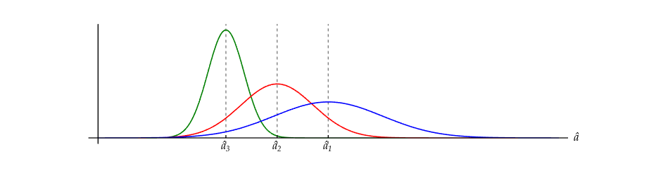
In other words, we would like the error, as we continue to use more data in our estimate, to go to zero. Formally, we want \(\sigma _a^2 \to 0\) as the number of samples \(N \to \infty.\) That is, the variance (or its square root, the standard deviation) of the estimate should go to zero as the number of samples becomes very large. As the variance of the estimate goes to zero, we describe the estimate as becoming more precise. If in the limit as \(N \to \infty\) both the bias and the variance go to zero, we say that the estimate is consistent2. This type of behavior is illustrated in Figure 11.1.
A convenient way to remember the concepts of accuracy and precision and to distinguish between them is through a (hypothetical) game of darts where the goal is to throw \(N\) darts such that each one lands in the center of the dart board, in the “bullseye”. This is illustrated in Figure 11.2.

The “intuitive” meanings of the words accurate and precise are illustrated here and intended to serve as a permanent reminder.
Estimating the mean
As an example consider \({m_x} = E\left\{ {x[n]} \right\}.\) We look at the arithmetic estimate for \({m_x}\) given by:
| (11.16) |
$$< x[n] > \; = \frac{1}{N}\sum\limits_{n = 0}^{N - 1} {x[n]}$$
|
We determine the bias as follows:
| (11.17) |
$$E\left\{ { < x[n] > } \right\}\; = \frac{1}{N}\sum\limits_{n = 0}^{N - 1} {E\left\{ {x[n]} \right\}} = {m_x}$$
|
| (11.18) |
$$B = E\left\{ { < x[n] > } \right\} - {m_x} = {m_x} - {m_x} = 0$$
|
Thus the arithmetic mean generates an unbiased estimate of the true mean. The variance, \(Var( \bullet ),\) of the estimate is:
| (11.19) |
$$\sigma _N^2 = Var\left\{ {\frac{1}{N}\sum\limits_{n = 0}^{N - 1} {x[n]} } \right\} = \frac{1}{{{N^2}}}\sum\limits_{n = 0}^{N - 1} {Var\left\{ {x[n]} \right\}}$$
|
This right-most term follows from the assumption that the data samples \(\{ x[n]\}\) are statistically independent of one another. Continuing,
| (11.20) |
$$\sigma _N^2 = \frac{1}{{{N^2}}}\sum\limits_{n = 0}^{N - 1} {\sigma _x^2} = \frac{1}{{{N^2}}}N\sigma _x^2 = \frac{{\sigma _x^2}}{N}$$
|
Thus, as the number of samples \(N \to \infty,\) the variance of the estimate goes to zero as \(1/N.\) Because the bias \(B\) is zero and the variance goes to zero for large \(N,\) we see that the estimate for the mean of a random process based upon Equation 11.16 is a consistent estimate.
An illustration of how the estimate shown in Figure 11.1 converges to a final value is shown in Movie 11.1.
Estimating the autocorrelation function
We now look at a more difficult problem, that of estimating the autocorrelation function of a real, random process starting from statistically independent data samples. Formally,
| (11.21) |
$${\varphi _{xx}}[k] = E\left\{ {x[n]{x^*}[n + k]} \right\} = \;E\left\{ {x[n]x[n + k]} \right\}$$
|
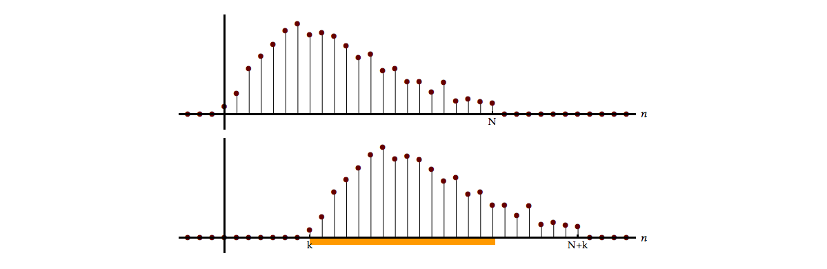
If \(N\) samples of \(\{ x[n]\}\) are available then only \(N - |k|\) samples are available to compute the average of the product \(x[n]\,x[n + k].\) This is illustrated graphically in Figure 11.3 and represents the fact that the number of overlaps between \(x[n]\) and \(x[n + k]\) will be \(N - \left| k \right|.\)
A dynamic rendering of the overlap that occurs during the calculation of the correlation is shown in Movie 11.2.
To estimate the mean of a parameter, we will use our result above, Equation 11.16, applied to:
| (11.22) |
$${c_{xx}}[k] = \frac{1}{{N - \left| k \right|}}\sum\limits_{n = 0}^{N - \left| k \right| - 1} {x[n]x[n + k]}$$
|
The variable \(k\) can be positive or negative but there will still be only \(N - \left| k \right|\) overlaps.
How good is our estimator?
The estimate of \({\varphi _{xx}}[k]\) is \({c_{xx}}[k].\) Our first question is: Is this estimate unbiased? The bias is given by:
| (11.23) |
$$B = E\left\{ {{c_{xx}}[k]} \right\} - {\varphi _{xx}}[k]$$
|
Using Equation 11.23:
| (11.24) |
$$\begin{array}{*{20}{l}}
B&{ = E\left\{ {\frac{1}{{N - \left| k \right|}}\sum\limits_{n = 0}^{N - \left| k \right| - 1} {x[n]x[n + k]} } \right\} - {\varphi _{xx}}[k]}\\
{\,\,\,}&{ = \frac{1}{{N - \left| k \right|}}\sum\limits_{n = 0}^{N - \left| k \right| - 1} {E\left\{ {x[n]x[n + k]} \right\}} - {\varphi _{xx}}[k]}\\
{\,\,\,}&{ = \frac{1}{{N - \left| k \right|}}\sum\limits_{n = 0}^{N - \left| k \right| - 1} {{\varphi _{xx}}[k]} - {\varphi _{xx}}[k]}
\end{array}$$
|
If \(\left| k \right| < N\) we have \(B = 0,\) an unbiased estimate. Our next question concerns the issue of whether \({c_{xx}}[k]\) forms a consistent estimate of \({\varphi _{xx}}[k].\) Since we know that the estimate is unbiased, it remains to be shown that the variance of the estimate goes to zero as the number of data samples \(N\) increases. The variance of the estimate, \(Var\{ {c_{xx}}[k]\},\) is given (for large \(N\)) by:
| (11.25) |
$$\begin{array}{*{20}{l}}
{Var\{ {c_{xx}}[k]\} \approx \frac{N}{{{{\left( {N - \left| k \right|} \right)}^2}}}\, \times }\\
{\,\,\,\,\,\,\,\,\,\,\,\,\,\,\,\left( {\sum\limits_{m = - \infty }^{ + \infty } {\left( {\varphi _{xx}^2[m] + {\varphi _{xx}}[m + k]{\varphi _{xx}}[m - k]} \right)} } \right)}
\end{array}$$
|
where formal derivation of the term under the summation is too complicated (and tedious) to be worked out in detail here; see Bartlett3 and Jenkins4, instead. We now define a function
| (11.26) |
$$\Phi [k] = \sum\limits_{m = - \infty }^{ + \infty } {\left( {\varphi _{xx}^2[m] + {\varphi _{xx}}[m + k]{\varphi _{xx}}[m - k]} \right)}$$
|
which leads to:
| (11.27) |
$$Var\{ {c_{xx}}[k]\} \approx \frac{N}{{{{\left( {N - \left| k \right|} \right)}^2}}}\Phi [k]$$
|
Let us look at \(\Phi [k]\) in more detail. It consists of two terms:
| (11.28) |
$$\Phi [k] = \sum\limits_{m = - \infty }^{ + \infty } {\varphi _{xx}^2[m]} + \sum\limits_{m = - \infty }^{ + \infty } {{\varphi _{xx}}[m + k]{\varphi _{xx}}[m - k]}$$
|
The first term, assuming it converges, is a positive, real number and independent of \(k.\) The remark that it is real follows from our assumption at the beginning of a section in Chapter 11. The second term is even in \(k\) as a simple substitution of \(- k\) shows. This means that \(\Phi [k]\) is even.
Further, the second term is itself an autocorrelation. Remembering our remarks at the beginning of Chapter 5, the second term is the autocorrelation of the deterministic correlation function with itself! Using Equation 6.32, this means the maximum value of \(\Phi [k]\) is given by:
| (11.29) |
$${\Phi _{\max }} = 2\sum\limits_{m = - \infty }^{ + \infty } {\varphi _{xx}^2[m]} \,\, \ge \,\,\Phi [k]\,\,\,\,\,\,\,\,\,\,\,\,\,\,\left| k \right| < N$$
|
Other aspects of \(\Phi [k]\) will be considered in Problem 11.9.
To better appreciate the behavior of \(\Phi [k]\) and how that influences the variance of the estimate of the autocorrelation function \(Var\{ {c_{xx}}[k]\},\) let us look at one specific example.
Langevin redux
In our case-study of the Langevin equation we saw in Equation 7.14 that the theory-based autocorrelation function for the stochastic velocity process was given by:
| (11.30) |
$${\varphi _{vv}}[k] = {\left( {\frac{1}{m}} \right)^2}\left( {\frac{{{F_o}}}{{1 - {\rho ^2}}}} \right){\rho ^{\left| k \right|}} = \frac{A}{{1 - {\rho ^2}}}{\rho ^{\left| k \right|}}$$
|
where \(0 < \rho = {e^{ - \lambda {T_s}/m}} < 1\) and the constant \(A = {F_o}/{m^2}.\) Velocity data collected from this type of study would then represent the basis for estimating \({\varphi _{vv}}[k].\) What can we expect from \({\Phi _{vv}}[k],\) the velocity example of \(\Phi [k],\) based upon this Langevin assumption?
This first term in Equation 11.28 can be computed directly and the result for \({\Phi _{vv}}[k]\) becomes:
| (11.31) |
$${\Phi _{vv}}[k] = \frac{{{A^2}(1 + {\rho ^2})}}{{{{(1 - {\rho ^2})}^3}}} + \sum\limits_{m = - \infty }^{ + \infty } {{\varphi _{vv}}[m + k]{\varphi _{vv}}[m - k]} $$
|
Understanding the behavior of the second term can be gained by first plotting the various components \({\varphi _{vv}}[m + k],\) \({\varphi _{vv}}[m - k],\) and \({\varphi _{vv}}[m + k]{\varphi _{vv}}[m - k].\) This is illustrated in Figure 11.4.

It is clear from Figure 11.4 that \({\varphi _{vv}}[m + k]{\varphi _{vv}}[m - k]\) is even in \(k\) and even in \(m.\) The former has already been proven; the latter will be proven in Problem 11.9. A consequence of the even symmetry is that to find \({\Phi _{vv}}[k]\) we need only solve the problem for \(k \ge 0.\)
For \(0 \le k \le m,\) we have \(m \pm k \ge 0\) and it follows that:
| (11.32) |
$$\begin{array}{*{20}{l}}
{{\varphi _{vv}}[m + k]{\varphi _{vv}}[m - k]}&{ = {{\left( {\frac{A}{{1 - {\rho ^2}}}} \right)}^2}{\rho ^{\left| {m + k} \right|}}{\rho ^{\left| {m - k} \right|}}}\\
{\,\,\,}&{ = {{\left( {\frac{A}{{1 - {\rho ^2}}}} \right)}^2}{\rho ^{m + k}}{\rho ^{m - k}} = {{\left( {\frac{A}{{1 - {\rho ^2}}}} \right)}^2}{\rho ^{2m}}}
\end{array}$$
|
This is a constant independent of \(k\) and explains the “flat behavior” observed for \(0 \le k \le m\) in Figure 11.4.
Following replacement of \(\left| {m - k} \right|\) with \(\left| {k - m} \right|\) and for \(0 \le m \le k,\) we have \(k \pm m \ge 0.\) It follows that:
| (11.33) |
$$\begin{array}{*{20}{l}}
{{\varphi _{vv}}[m + k]{\varphi _{vv}}[m - k]}&{ = {{\left( {\frac{A}{{1 - {\rho ^2}}}} \right)}^2}{\rho ^{\left| {k + m} \right|}}{\rho ^{\left| {k - m} \right|}}}\\
{\,\,\,}&{ = {{\left( {\frac{A}{{1 - {\rho ^2}}}} \right)}^2}{\rho ^{k + m}}{\rho ^{k - m}} = {{\left( {\frac{A}{{1 - {\rho ^2}}}} \right)}^2}{\rho ^{2k}}}
\end{array}$$
|
This is an exponentially decreasing function for \(k > 0\) and explains the behavior observed for \(0 \le m \le k\) in Figure 11.4.
To continue, we deconstruct the sum in Equation 11.31 for \(k \ge 0\) as follows:
| (11.34) |
$$\begin{array}{l}
\sum\limits_{m = 0}^{ + \infty } {{\varphi _{vv}}[m + k]{\varphi _{vv}}[m - k]} = \underbrace {{\varphi _{vv}}[k]{\varphi _{vv}}[k]}_{m = 0}\,\, + \\
\,\,\,\,\,\,\,\,\,\underbrace {\sum\limits_{m = 1}^k {{\varphi _{vv}}[m + k]{\varphi _{vv}}[m - k]} }_{0 < m \le k}\,\,\, + \\
\,\,\,\,\,\,\,\,\,\,\,\,\,\,\,\,\,\,\,\underbrace {\sum\limits_{m = k + 1}^{ + \infty } {{\varphi _{vv}}[m + k]{\varphi _{vv}}[m - k]} }_{k < m \le \infty }
\end{array}$$
|
Substituting the various terms we have already found:
| (11.35) |
$$\begin{array}{l}
\sum\limits_{m = 0}^{ + \infty } {{\varphi _{vv}}[m + k]{\varphi _{vv}}[m - k]} = \underbrace {{{\left( {\frac{A}{{1 - {\rho ^2}}}} \right)}^2}{\rho ^{2k}}}_{m = 0}\,\, + \\
\,\,\,\,\,\,\,\,\,\,\,\,\,\,\,\,\,\,\,\underbrace {\sum\limits_{m = 1}^k {{{\left( {\frac{A}{{1 - {\rho ^2}}}} \right)}^2}{\rho ^{2k}}} }_{0 < m \le k} + \underbrace {\sum\limits_{m = k + 1}^{ + \infty } {{{\left( {\frac{A}{{1 - {\rho ^2}}}} \right)}^2}{\rho ^{2m}}} }_{k < m \le \infty }
\end{array}$$
|
The two sums in Equation 11.35 converge yielding for \(k \ge 0\):
| (11.36) |
$$\begin{array}{l}
\sum\limits_{m = 0}^{ + \infty } {{\varphi _{vv}}[m + k]{\varphi _{vv}}[m - k]} = {\left( {\frac{A}{{1 - {\rho ^2}}}} \right)^2}{\rho ^{2k}}\,\, + \\
\,\,\,\,\,\,\,\,\,\,\,\,\,\,\,\,\,\,\,{\left( {\frac{A}{{1 - {\rho ^2}}}} \right)^2}k{\rho ^{2k}} + {\left( {\frac{A}{{1 - {\rho ^2}}}} \right)^2}\frac{{{\rho ^{2(k + 1)}}}}{{1 - {\rho ^2}}}
\end{array}$$
|
Combining the even term for \(k < 0\) gives the final result:
| (11.37) |
$$\begin{array}{l}
{\Phi _{vv}}[k] = \frac{{{A^2}(1 + {\rho ^2})}}{{{{(1 - {\rho ^2})}^3}}} + {\left( {\frac{A}{{1 - {\rho ^2}}}} \right)^2}{\rho ^{2\left| k \right|}}\,\, + \\
\,\,\,\,\,\,\,\,\,\,\,\,\,\,\,\,\,\,\,2{\left( {\frac{A}{{1 - {\rho ^2}}}} \right)^2}\left| k \right|{\rho ^{2\left| k \right|}} + 2{\left( {\frac{A}{{1 - {\rho ^2}}}} \right)^2}\frac{{{\rho ^{2(\left| k \right| + 1)}}}}{{1 - {\rho ^2}}}
\end{array}$$
|
Rewriting these terms yields:
| (11.38) |
$$\begin{array}{l}
{\Phi _{vv}}[k] = \frac{{{A^2}}}{{{{(1 - {\rho ^2})}^3}}}\,\,\, \times \\
\,\,\,\,\,\,\,\,\,\,\,\,\,\,\,\,\,\,\,\left( {1 + {\rho ^2} + (1 - 2\left| k \right|){\rho ^{2\left| k \right| + 2}} + (1 + 2\left| k \right|){\rho ^{2\left| k \right|}}} \right)
\end{array}$$
|
In Figure 11.5 we show the behavior of the function \({\Phi _{vv}}[k]\) for several values of the parameter \(\rho.\)

This continuation of the case study of the Langevin equation that was begun in Chapter 7 shows how the estimation of an important descriptor of that random process, the autocorrelation function, can be analyzed. The differential equation—and hence the resulting difference equation—was first order. See Equation 7.1 and Equation 7.5. As a consequence the results presented here are applicable for most first-order processes.
Trouble in paradise
We return to our general remarks concerning the variance of the estimate of the autocorrelation function. If \(\Phi [k]\) is bounded (as in the above example with \({\Phi _{\max }}\) from Equation 11.29), that is, if \(\left| {\Phi [k]} \right| < \infty\) for all \(\left| k \right| < N,\) we might think that Equation 11.27 implies that the variance goes to zero as \({N^{ - 1}}.\) This, however, is not true for all values of \(k.\) As \(\left| k \right| \to N\) the variance diverges (blows-up) independent of how large \(N\) is! Thus the estimate given in Equation 11.22 is not consistent.
We might try, instead, a different estimate of the autocorrelation function. Specifically,
| (11.39) |
$$\begin{array}{*{20}{l}}
{{{\hat c}_{xx}}[k]}&{ = \frac{1}{N}\sum\limits_{n = 0}^{N - \left| k \right| - 1} {x[n]x[n + k]} }\\
{\,\,\,}&{ = \left( {\frac{{N - \left| k \right|}}{N}} \right){c_{xx}}[k]}
\end{array}$$
|
The simple relation between the two estimates for \({\varphi _{xx}}[k]\) gives:
| (11.40) |
$$E\left\{ {{{\hat c}_{xx}}[k]} \right\} = \left( {\frac{{N - \left| k \right|}}{N}} \right){\varphi _{xx}}[k]$$
|
Clearly \({\hat c_{xx}}[k]\) is a biased estimate, an underestimate. The variance, however, is
| (11.41) |
$$Var\{ {\hat c_{xx}}[k]\} = {\left( {\frac{{N - \left| k \right|}}{N}} \right)^2}Var\{ {c_{xx}}[k]\} = \frac{1}{N}\Phi$$
|
which converges to zero as \(N \to \infty.\) We are faced with a choice: if we choose \({c_{xx}}[k]\) we have an estimate of \({\varphi _{xx}}[k]\) that is unbiased but blows up (diverges) as \(\left| k \right| \to N.\) This occurs because as \(\left| k \right|\) approaches \(N,\) there are very few overlapping data samples—see Movie 11.2—and thus the variance associated with the estimate is large. If we choose \({\hat c_{xx}}[k]\) we have an estimate that converges nicely as \(N \to \infty\) but is biased; it is an underestimate. Such a trade-off between desired properties is not uncommon in the estimation of parameters of stochastic signals.
In this chapter we have looked at the estimation of the mean Equation 11.1 and the correlation function Equation 11.2. In the next chapter we will consider the problem of estimating the power spectral density Equation 11.3.
Problems
Problem 11.1
We are given a function of \(x\) that is non-negative, that is, \(f(x) \ge 0\) for all \(x.\)
Show that the values of \(x\) for which \(\ln \left( {f(x)} \right)\) has an extremum are also values of \(x\) where \(f(x)\) has an extremum.
Problem 11.2
The Gaussian (normal) probability density function is given by:
Determine a maximum-likelihood estimate for \(\mu\) given \(N\) data samples \(\left\{ {{x_1},{x_2},...,{x_N}} \right\}.\) Assume that \(\sigma\) is known.
Problem 11.3
We wish to determine if a coin is “fair”. We flip the coin \(N\) times at 10:00 in the morning and write down the number of “Heads” \(n.\) We then repeat this process for \(M\) days.
- What is the ML-estimate for the probability of Heads, \(p = p(Heads)?\)
- Why might the time of performing this experiment be relevant?
Problem 11.4
The probability density function for the emission of the first photon from a fluorescent sample in the time interval \((0,t)\) is given by:
We have a series of independent measurements for the emission times of first photons from identical molecules \(\left\{ {{t_1},{t_2},{t_3},...,{t_N}} \right\}.\)
- Determine the ML-estimate for \(\lambda.\)
- What is the relation between \({\lambda _{ML}}\) from part (a) and the harmonic mean given in Equation 11.6?
Problem 11.5
Let a random process have a parameter—for example the mean or variance—whose true (non-random) value is \(a\) and whose estimate is \(\hat a.\) The mean-square error associated with this estimate is given by \(e\):
| (11.42) |
$$e = E\left\{ {{{\left( {\hat a - a} \right)}^2}} \right\}$$
|
Let \({\tilde a}\) be the unbiased estimate of \(a,\) that is \(B = E\left\{ {\tilde a} \right\} - a = 0.\)
Show that if the goal is to minimize the mean-square error \(e,\) then the best estimate for \(a\) is the unbiased estimate, that is \(\hat a = \tilde a.\) Hint: Consider replacing \({\left( {\hat a - a} \right)}\) with \(\left( {\hat a - \tilde a + \tilde a - a} \right).\)
Problem 11.6
We know from Equation 4.18 that for any random variable \(\theta\) where the mean and variance exist (that is, are finite) we have \(Var\left( \theta \right) = E\left\{ {{\theta ^2}} \right\} - {\left( {E\left\{ \theta \right\}} \right)^2}.\) If \({\theta _o}\) is the true value of a parameter of a distribution, such as the mean or variance, and \(\theta\) is an estimate of \({\theta _o}\) based upon collected data, then \(\theta - {\theta _o}\) is also a random variable and we have:
| (11.43) |
$$Var(\theta - {\theta _o}) = E\left\{ {{{(\theta - {\theta _o})}^2}} \right\} - {\left( {E\left\{ {\theta - {\theta _o}} \right\}} \right)^2}$$
|
Use this to show that:
| (11.44) |
$$e = Var(\theta ) + {B^2}(\theta )$$
|
where, as in Equation 11.42, \(e\) is the mean square error in the estimate of \(\theta\) and \(B\) is the bias in the estimate. Hint: This might be a good time to review Problem 4.4.
Problem 11.7
Consider an ergodic Gaussian random process \(x\) which, without loss of generality, is standardized. That is, \({\mu _x} = 0\) and \({\sigma _x} = 1.\) (See Problem 4.9.) We wish to estimate the variance of this process based upon \(N\) samples. We propose an estimator of the form:
| (11.45) |
$$s_x^2 = \frac{1}{K}\sum\limits_{n = 1}^N {{{\left( {{x_n} - < x > } \right)}^2}}$$
|
where \(< x >\) is the arithmetic mean Equation 11.4 of the \(N\) samples of \(x.\) In this problem we will explore the consequences of choosing different values for \(K.\)
It can be shown that:
| (11.46) |
$$\frac{1}{{\sigma _x^2}}\sum\limits_{n = 1}^N {{{\left( {{x_n} - < x > } \right)}^2}}$$
|
is a Chi-squared (\({\chi ^2}\)) distributed random variable with \(N - 1\) degrees-of-freedom (dof); see Cramér5. The mean and variance of a \({\chi ^2}\) distributed random variable are dof and 2•dof, respectively.
- Determine the bias \(B\) associated with the estimate for the variance \(\sigma _x^2.\)
- How should Equation 11.45 be modified if the estimate is to be unbiased, that is, \(B = 0?\)
- What is the variance associated with the estimate in Equation 11.45? What does this become if the unbiased version of Equation 11.45 is used?
- Is the unbiased estimate of the variance a consistent estimator?
- Using Equation 11.44, what value of \(K\) in Equation 11.45 yields a minimum mean-square error \(e?\) Is this the same value of \(K\) that you found for an unbiased estimate in part (b) of this problem?
- Is Equation 11.45 a minimum-variance unbiased estimator (MVUE)?
Problem 11.8
The real, ergodic, stochastic signal \(x[n]\) is characterized by a mean value of \({m_x} = < x[n] > = 0\) and an autocorrelation \({\varphi _{xx}}[k] = < x[n]{x^*}[n + k] >.\) Let \(y[n] = A \bullet x[n]\) where \(A\) is a constant to be determined.
- Find the value of \(A\) that minimizes \({\varphi _{ee}}[k]\) where \(e[n] = y[n] - x[n - N]\) for a fixed value of \(N.\) That is, we wish \(y[n]\) to be a least-mean-square predictor of \(x[n]\) and \(e[n]\) represents the error in the prediction at any given time.
Discuss your result for the two extreme cases:
Problem 11.9
We have from Equation 11.26 that:
| (11.47) |
$$\begin{array}{*{20}{l}}
{\Phi [k]}&{ = \sum\limits_{m = - \infty }^{ + \infty } {\left( {\varphi _{xx}^2[m] + {\varphi _{xx}}[m + k]{\varphi _{xx}}[m - k]} \right)} }\\
{\,\,\,}&{ = \sum\limits_{m = - \infty }^{ + \infty } {\varphi _{xx}^2[m]} + \sum\limits_{m = - \infty }^{ + \infty } {{\varphi _{xx}}[m + k]{\varphi _{xx}}[m - k]} }
\end{array}$$
|
- Assume that the random variable \(x\) is real. Using Equation 5.5 prove that \({{\varphi _{xx}}[m + k]{\varphi _{xx}}[m - k]}\) is even in \(m.\)
- As indicated in the text, the second term, which has the form \(\sum {{\varphi _{xx}}[m + k]{\varphi _{xx}}[m - k]},\) is an autocorrelation function. Let us call it \({\psi _{xx}}[k].\) Determine the power spectral density \({S_{\psi \psi }}(\Omega ) = {\mathscr{F}}\left\{ {{\psi _{xx}}[k]} \right\}\) in terms of \({S_{xx}}(\Omega )\) and \(X(\Omega ).\)
- Determine the maximum value of \({\Phi _{vv}}[k],\) the complicated term involved in the variance of the estimate of the autocorrelation function of the Langevin velocity process. Your result should be in terms of \(A\) and \(\rho.\) You might also want to review Chapter 7 and Chapter 7.
- You are required to keep \(N\) and \(k\) constant in Equation 11.25 and you wish to decrease the variance of your estimate of the autocorrelation function of the Langevin velocity process in part (c). Should you raise or lower the temperature \(\Psi\) at which an experiment is performed? Does your mathematical result agree with your physical intuition? Explain your reasoning. Again, you might want to review Chapter 7.
Problem 11.10
Show that for \(0 < m \le k\) that the term \({\varphi _{vv}}[m + k]{\varphi _{vv}}[m - k]\) in Equation 11.31 becomes:
| (11.48) |
$${\varphi _{vv}}[m + k]{\varphi _{vv}}[m - k] = {\left( {\frac{A}{{1 - {\rho ^2}}}} \right)^2}{\rho ^{2k}}$$
|
Hint: Use the evenness properties of Problem 11.9.
Laboratory Exercises
Laboratory Exercise 11.1
|
There is more than just one “mean”. And depending upon the nature of an estimation problem, one may be more suitable than another. That is no mean feat. To start the exercise, click on the icon to the left. |
Laboratory Exercise 11.2

|
Is precision the same as accuracy? Answer the question now and then answer the question after the exercise. To start the exercise, click on the icon to the left. |
Laboratory Exercise 11.3

|
Can you measure a distance of 1 mm with a ruler that is only marked in centimeters? Or how about the length of a bridge that is less than a mile long with an odometer that only reports whole (integer) miles? To start the exercise, click on the icon to the left. |
-
van den Bos, A. (2007). Parameter Estimation for Scientists and Engineers. Hoboken, New Jersey, Wiley-Interscience ↩
-
The usual definition of “consistent” involves the convergence in probability of the estimate. By using the Tchebyshev inequality in probability theory it can be shown that the two definitions are equivalent. ↩
-
Bartlett, M. S. (1946). “On the theoretical specification and sampling properties of autocorrelated time series.” Journal of the Royal Statistical Society Suppplement, Vol. 8(1) ↩
-
Jenkins, G. M. and D. G. Watts (1998). Spectral Analysis and Its Applications, Emerson Adams Press ↩
-
Cramér, H. (1946). Mathematical Methods of Statistics. Princeton, New Jersey, Princeton University Press, Section 18.1 ↩